Optimal Load Factor for Approximate Nearest
Neighbor Search under Exact Euclidean Locality
Sensitive Hashing
Ruben Buaba
Autonomous Control and Information Technology Center,
Department of Electrical and Computer Engineering North Carolina Agricultural and
Technical State University Greensboro, NC 27411
Abdollah Homaifar
Autonomous Control and Information Technology Center,
Department of Electrical and Computer Engineering North Carolina Agricultural and
Technical State University Greensboro, NC
Eric Kihn
NOAA /NGDC 325 Broadway Boulder,CO
80305
ABSTRACT
Locality Sensitive Hashing (LSH) is an index-based data structure that allows spatial item retrieval over a large dataset. The performance measure, ρ, has significant effect on the computational complexity and memory space requirement to create and store items in this data structure respectively. The minimization of ρ at a specific approximation factor c, is dependent on the load factor, α. Over the years,𝛼 = 4has been used by researchers. In this paper, we demonstratethat the choice of𝛼 = 4does not guarantee low computational complexity and low memory space of the data structure under the LSH scheme. To guarantee low computational complexity and low memory space, we propose𝛼 = 5. Experiments on the Defense Meteorological Satellite Program imagery datasethave shown that𝛼 = 5saves more than 75%on memory space; cuts the computational complexity by more than 70%andanswers query two times faster on the average compared to that of𝛼 = 4.
General Terms
Nearest Neighbor, Search Algorithm, Locality Sensitive Hashing
Keywords
Approximate Nearest Neighbor, Exact Nearest Neighbor, ApproximationFactor, Performance Measure,Optimal Load Factor
1.
INTRODUCTION
1.1
Nearest Neighbor Search
A nearest neighbor (NN) search is composed as follows: given a setP of n data pointsin a metric space, X, the task is to preprocess these points sothat, given any query point𝒒 ∈Pthe data point nearest to qcan be reported quickly. This is also referred to as the closest-pointproblem or the post office problem[1]. Even though linear search (LS) algorithm guarantees the retrieval of the exact nearest data point to a given query point correctly, it becomes computationally exhaustive and queryruntime complexity can be exponential when dealing with a large datasetwithhigh dimensionality. The reason being,LS literally iterates through the entire dataset and computes some metric distance between each data point and the query point and then returns the data point closest to the query point.
In practice, the NN search problem involves a collection of large number of items characterized by high dimensionality. In reality, the dataset for most applications is dynamic. In other words, the dataset is updated as when new data is collected. Consequently, similarity search algorithm should scale to produce an output within a reasonable timespan irrespective of the growth of the dataset. Thus, building a data structure that can be used to index and store these items in such a manner that given any query item, the search algorithm is able to find the most similar itemin sublinearquery runtime is vital. This problem is of major importance including but not limited to image and video database retrieval, data compression, information retrieval, database and data mining, pattern recognition, statistics and data analysis[2, 3].
Over the years, intensive research has been done either to use trees, K-means clustering/classification or hashes to develop a space-partitioned data structure that would have a sublinearquery runtime[4-8]. For uniformly distributed data points, expected query runtime is achievable by algorithms that decompose the search space into regular grids [9, 10]. In [11], the authors generalized these results and reported that
in 𝑂(log 𝑛) time with 𝑂(𝑛 𝑑 2 +𝛿)space with hidden constant factors that are exponential in d. In [19], the authors generalized this by providing a trade-off between space and query runtime. Later in[20], it is reported that exponential factors in query runtime could be eliminated with an algorithm having 𝑂(𝑑5log 𝑛) query time and 𝑂(𝑛𝑑+𝛿) space. Unfortunately, it is shown both theoretically and empiricallythat these solutions provide little or no improvement over the LS algorithm for highly dimensional large dataset[21, 22]. Consequently, several researchers have become proponents of the use of approximation similarity search algorithms[23-27]. The fundamental principle being, in practice, approximate nearest neighbor is almost as good as the exact nearest neighbor in most cases. Since a distance measure is what is often used for similarity estimation, a small difference in the distance should not adversely influence the similarity estimation unless the nearest neighbor problem itself is unstable[28, 29]. This notion of approximation forms the basis of a novel similarity search algorithm known as the Locality Sensitive Hashing (LSH) which was first introduced in[25]. This technique drastically reduces the query runtime at the expense of a small probability of failure to find the absolute closest match. The concept of the approximate
nearest neighbor (ANN) in some ls norm space is formulated
as follows: suppose q is a query whose exact NN is q*. For a given 𝑐 > 1, p is said to be a c-NN of q if 𝒑 − 𝒒 𝑠≤
𝑐 𝒑 − 𝒒∗ 𝑠.
The performance of LSH depends on the minimization ofthe performance measure,ρ that is associated with an optimal load factor α.This guides the memory requirement, the computational complexity and the query runtime of the data structure under the LSH scheme. Over the years, many researchers haveused 𝛼 = 4[25, 21, 30, 31]. In this paper, it is demonstrated that the choice of 𝛼 = 4 does not guarantee low memory requirement and low computational complexity of the data structure under the LSH scheme. In addition, the query runtime is slow. We show that under the LSH scheme, a load factor of𝛼 = 5guarantees a lower memory requirement, lowercomputational complexity and faster query runtime compared to the conventional choiceof 𝛼 = 4.
The remainder of this paper is organized as follows: Section 1.2 formulates the problem; section 2 offers the background of LSH in general; section 3 explains theorems and parametric constraintsof our proposed technique; section 4 talks about the complexity of the LSH; section 5 offers an empirical implementation of LSH on real data; and section 6draws the conclusions and proposes a future improvement.
1.2
Notations and Problem Definition
Unless otherwise stated the following parameter notations are used throughout this paper. P is a set of n data points in d-dimensional space (ℜ𝑑). A query data point and any other point are denoted q and p respectively such that 𝒑 ≠ 𝒒 ∈P. A sphere of radius R centered at q is denoted by 𝛽(𝒒, 𝑅). For any 𝜀 > 0, 𝑐 = 1 + 𝜀 is the approximation factor such that
𝑐𝑅 > 𝑅. The l2 norm of p is denotedby 𝑝 2. The expected
number of data points per bucket (i.e. load factor) is denoted byα. Our goal is to build a data structure forP under the LSH scheme by choosing an optimal value forαthat guarantees lower memory, lowercomputational complexityand faster query runtime than that of the existing load factor,𝛼 = 4.This data structure is to solve the (R, c)-nearest neighbor problem in the l2 norm space defined as follows: if ∃ 𝒒∗: 𝒒 − 𝒒∗ 2≤
𝑅 then in sublinearquery runtime, report any point 𝒑: 𝒒 −
𝒑 2≤ 𝑐𝑅 if it such a point exists.
2.
LSH BACKGROUND
LSH is an index-based data structure that allows spatial item retrieval over a large database. The basic idea underlying the operation and the effectiveness of the LSH is that if two data points 𝒑, 𝒒 ∈ ℜ𝑑 (i.e. 𝑑 ∈ 𝑍+) are close, then after a scalar projection of these points onto a hyper-plane, the two points should remain close to each other. On the other hand, if the points are far apart, they should remain far apart from each other after a scalar projection onto that same hyper-plane. This assertion is true in most cases[25, 32].However, with small failure probability,δ, some points that are far apart might become closer after projection onto a lower dimension. For a dynamic dataset (i.e. dataset grows from time to time), the major advantage of LSH over tree-data structures is its ability to support deletion and insertion [30] operations. Suppose the real number line is "chopped" into slots (i.e. bucket)numbered 0, 1, … , 𝑚 − 1 to form a table. If integer values are assigned to the data points based on which slots they project to, then intuitively, making several projections certainly increases the probability,P1 of nearby points
projecting to the same slot and decrease the probability, P2 of
far points from projecting to same slot. To make further guarantee this, several families of hash functions are used to perform the scalar projections. To achieve this goal, the functions must be locality sensitive and universal[33].
Definition #1: A family of hash functions, ℋ = {𝒉𝒊𝒋:P→ 𝑈} each hij mapping one point from domainPto domain U, is said
to be 𝑃1> 𝑃2, 𝑐𝑅 > 𝑅locality-sensitive if for any 𝒑, 𝒒 ∈P,
if 𝒑 ∈ 𝛽(𝒒, 𝑅) then Pr[𝑖𝑗 𝒑 = 𝑖𝑗(𝒒)] ≥ 𝑃1(′𝑖𝑔′) if 𝒑 ∉ 𝛽(𝒒, 𝑐𝑅) then Pr[𝑖𝑗 𝒑 = 𝑖𝑗(𝒒)] ≤ 𝑃2(′𝑙𝑜𝑤′)
Definition #2: Suppose P is a universe of keys, and ℋis a family of a finite collection of hash functions, each mapping Uto 0,1, … , 𝑚 − 1, ℋ is said to be universal if ∀ 𝒑, 𝒒 ∈
Pand 𝑝 ≠ 𝑞, then Pr 𝑖𝑗∈ ℋ: 𝑖𝑗 𝒑 = 𝑖𝑗 𝒒 = ℋ/m.
A well-developed hash function tries to amplify the gap between the two probabilities,
P
1andP
2. To guarantee this amplification 𝑃1/𝑃2, k hash functions are chosen identicallyand independently from ℋ. To further amplify the gap between P1 and P2, Ltables are created. Whenever two or
more items hash into the same bucket on any table, collision, is said to have occurred and this is sometimes resolved using double hashing, linked-list, or chaining. Normally, the number of buckets is large. As a result, it is only the non-empty buckets that are retained after all the data points in Pare projected into the buckets on the various tables. Creation of hash tables is normally fast and simple if the objects in the dataset are binary strings, i.e. 0 1 𝑑[21, 25]— the biggest drawback of LSH. In spite of this limitation, LSH algorithm has been used in a number of applications involving non-binary data set[34-40]. To handle non-binary dataset, the algorithm has to be extended to the l2 norm, by embedding l2
space into l1 space, and then l1 space into the binary Hamming
space. This however increases the complexity of the search algorithm but the advantages achieved outweigh this drawback.
Once the hash table is created and stored, for any query point 𝒒 ∈P, the 𝑅, 𝑐 -NNs can be found by hashing qand retrieving data points stored in the buckets
between a larger table with a smaller final linear search or a more compact table with more data points to consider in the final search. The 𝑅, 𝑐 -NNs search is terminated after finding the first 2L data points (including duplicates) closet to q[30]. The parameters k and L are chosen such that the following two conditions hold with constant probabilities: Condition #1: if 𝒒∗∈ 𝛽(𝒒, 𝑅), then𝑗 𝒒∗ = 𝑗(𝒒)for
some 𝑗 = 1,2, … , 𝐿
Condition #2: the expected number of collision of 𝒒 with any point 𝒑 ∈P such that 𝒑 ∈ 𝛽(𝒒, 𝑐𝑅) is less than 2L
3.
THEORY AND CONSTRAINTS
3.1
S-stable Distribution
Stable distributions are defined as limits of normalized sums of independent identically distributed variables [41]. A distribution Dis said to be s-stable if there exists 𝑠 ≥ 0, such that for any N real numbers 𝑢1, 𝑢2, … , 𝑢𝑁 and independent identically distributed random variables, 𝑋1, 𝑋2, … , 𝑋𝑁 with
distribution D, the random variable, 𝑁𝑖=1𝑢𝑖𝑋𝑖 has the same
distribution as the variable 𝑁𝑖=1 𝑢𝑖 𝑠 1/𝑠
𝑋, where X is a random variable with distribution D. For 𝑠 ∈ [0, 2], there exist stable distributions[41]. However, the focus is shifted to the case, 𝑠 = 2 since the similarity measure which is normally used is the l2 norm (the Euclidean space). Under this, the
normal Gaussian distribution denoted, 𝒩(0, 1) with a probability distribution function, 𝑓 𝑥 = 2𝜋1 𝑒−𝑥2/2 is 2-stable. Stable distributions have applications in many fields [34]. In computer science, stable distributions are used for "sketching" high dimensional vectors[25].
Suppose a random vector 𝒉𝒊𝒋∈ ℜ𝑑 is chosen from the standard Gaussian distribution, 𝒉𝒊𝒋~𝒩(0, 1) and 𝒑is any vector such that 𝒑 ∈ ℜ𝑑→ 𝒑 = [𝑝1, 𝑝2, … , 𝑝𝑑]. Then the scalar dot product 𝒉𝒊𝒋• 𝒑 is a random variable which tends to
be distributed as 𝒑 2𝒉𝒊𝒋, where hij is a random variable with
2-stable distribution and 𝑝 2 is the l2 norm of vector p given
as 𝑝 2= 𝑑𝑧=1𝑝𝑧2 1/2
. In other words, the difference,𝒉𝒊𝒋•
𝒑 − 𝒉𝒊𝒋• 𝒒 tends to be distributed as 𝒒 − 𝒑 2𝒉𝒊𝒋. Small collections of such dot products corresponding to different hijcan be used to estimate 𝒒 − 𝒑 2,the l2 norm between the
two data points 𝒑, 𝒒 ∈P. Hence the data structure under the LSH scheme is said to be l2-embedding and the l2 norm forms
the similarity metric for finding the NN to a given query data point.
3.2
Evaluation of P1 and P2
Suppose 𝑐 = 𝒒 − 𝒑 2 and bij is an offset drawn uniformly
from [0, 𝛼] at random. Also assume that hj is a family of k
hash functions drawn randomly and independently from
𝒩(0, 1) such that, 𝑗 = [𝒉𝟏𝒋, 𝒉𝟐𝒋, … , 𝒉𝒌𝒋]. The hash value of
𝒑 can be computed
as,𝑗 𝒑 = 𝒉𝟏𝒋•𝒑+𝑏𝛼 1𝑗 , 𝒉𝟐𝒋•𝒑+𝑏𝛼 2𝑗 , … , 𝒉𝒌𝒋•𝒑+𝑏𝛼 𝑘𝑗 .From the 2-stable distribution, 𝒉𝒊𝒋• 𝒑 − 𝒉𝒊𝒋• 𝒒 for any ith hash function
such 𝒉𝒊𝒋∈ 𝑗has the same distribution as𝑐𝒉𝒊𝒋. The probability
that 𝒑 and 𝒒collides is given by Equation (1). The 𝐹(•) in Equation(1) represents the probability density function of the absolute value of the Gaussian distribution.
Pr 𝑐 = Pr 𝑗 𝒑 = 𝑗 𝒒 = 0𝛼1𝑐𝐹 𝑡𝑐 1 −𝛼𝑡 𝑑𝑡(1)
It should be noted that for a given α, the probability of collision decreases monotonically with c. This means that the probability of collision is high if 𝒑 − 𝒒 2 is small and low if
𝒑 − 𝒒 2 is large. Thus, as per Definition#1, for this to be
𝑃1> 𝑃2, 𝑐𝑅 > 𝑅sensitive 𝑃1= Pr 𝑐 = 1 and 𝑃2= Pr 𝑐 > 1 . Solving these yieldEquations (2) and (3) with 𝐹𝑐𝑑𝑓(•) being the cumulative distribution function of the Gaussian random variable.
𝑃1= 1 − 2𝐹𝑐𝑑𝑓 −𝛼 − 2𝜋𝛼2 1 − 𝑒
−𝛼2 2
(2)
𝑃2= 1 − 2𝐹𝑐𝑑𝑓 −𝛼/𝑐 − 2𝜋𝛼/𝑐2 1 − 𝑒−𝛼2/2𝑐2 (3)
These prior probabilities influence the performance measure, ρ as shown in Equation (4).
𝜌 = ln 𝑃1 ln 𝑃2
(4)
3.3
Computing the performance measure, ρ
The two prior probabilities P1and P2are needed to compute ρ.From Equation(2), once α is known P1can be computed. To
compute P2 from Equation(3), both α and c must be known.
Theρ directly affects the memory space required to store items in the hash table. As a result, the goal is to find α that minimizes ρ at a specific c. In other words, the aim is to solve Equation(5).
min∀𝛼∈𝑍+ ln 𝑃1 ln 𝑃
2
(5)
There exists no closed-form solution for Equation(5). In [25], the authors provided an approximate solution as 𝜌(𝑐) ≈ 1/𝑐. A minimization tool such as Matlab could be used to find the optimal value for ρ. Later in[30], the authors conducted a minimization experiment in Matlab to solve Equation(5). The experiment was conducted for𝑐 = (1 10]in increment of 0.05. For each value of c, the minimum value of𝜌(𝑐)is computed over the range of α. They concluded that their approach gave a minimum value of ρ slightly below the approximate solution by[25]. Furthermore, they observed thatρ is not very sensitive to α beyond a certain point; and as long α is chosen “sufficiently” away from 0, the value ofρ would be close to optimal. They added that, if α is too large, both P1 and P2
approach unity and this increases memory space and the query runtime.
3.4
Proposed Optimal Load Factor
Over the years, researchers use 𝛼 = 4proposed by [30]as the optimal load factor. This however, raises two major concerns. First, does the choice of𝛼 = 4guarantee low computational complexityand low memory space to create and store a data structure for n data points under the LSH scheme? Second, assuming𝛼 = 4 is indeed the optimal load factor, what is the „best‟ optimal performance measure,ρ to choose if 𝛼 = 4gives multiple distinct values forρat different values of c? We address these concerns by repeating the same experiment by[30] after which a multi-objective optimization is used to find the actual optimalαandρ.
In our experiment over the same specified range for c, there is a statistical frequency count of the number of times a specific optimal load factor, 𝛼𝑜𝑝𝑡minimizes Equation(5) at different values of c to give different optimal values ofρ denoted
𝜌𝑜𝑝𝑡.Let this frequency be denotedby𝑓𝛼𝑜𝑝𝑡.Let Cαopt be a set
of the distinct values of c for that 𝛼𝑜𝑝𝑡such that𝑓𝛼𝑜𝑝𝑡 >
highest𝑓𝛼𝑜𝑝𝑡has the widest span of c in its corresponding set,
Cαopt. This means that the choice of such𝛼𝑜𝑝𝑡would support a
wider range of approximation factors. As per Definition #1, P1must be „high‟ and P2 must be „low‟. Thus, the final choice
of a specific 𝛼𝑜𝑝𝑡 depends not only on it having the highest
𝑓𝛼𝑜𝑝𝑡 but also on the corresponding c that maximizes P1, and
minimizes both P2and𝜌𝑜𝑝𝑡.The problem then becomes a
multi-objective optimization. Let P1opt and P2opt be the
optimal values of P1 and P2respectively. Also let ραopt be the
optimal value of𝜌𝑜𝑝𝑡.Suppose𝛼𝑜𝑝𝑡𝑀𝑎𝑥 is the optimal load factor with the highest frequency. Then,P1opt and ραopt can be
obtained using Equations (6) and (7) respectively.
𝑃1𝑜𝑝𝑡 = 1 − 2𝐹𝑐𝑑𝑓 𝛼𝑜𝑝𝑡𝑀𝑎𝑥 − 2𝜋𝛼2
𝑜𝑝𝑡𝑀𝑎𝑥 1 −
𝑒−𝛼𝑜𝑝𝑡𝑀𝑎𝑥
2
2 (6)
𝜌𝛼𝑜𝑝𝑡 = min ∀𝛼∈𝐶𝛼𝑜𝑝𝑡
ln 𝑃1𝑜𝑝𝑡
ln 𝑃2 𝑐 |𝛼=𝛼𝑜𝑝𝑡𝑀𝑎𝑥 (7)
Suppose ραopt is obtained at
c
c
opt
C
opt. Then, P2opt canbe computed either using Equation(8) or (9).
𝑃2𝑜𝑝𝑡 = 1 − 2𝐹𝑐𝑑𝑓 −𝛼𝑜𝑝𝑡
𝑐𝑜𝑝𝑡 −
2
2𝜋𝛼𝑜𝑝𝑡𝑐𝑜𝑝𝑡 1 − 𝑒 −𝛼2/2𝑐𝑜𝑝𝑡2
(8)
𝑃2𝑜𝑝𝑡 = 𝑒ln 𝑃1𝑜𝑝𝑡 𝜌𝛼𝑜𝑝𝑡
(9)
Figure1 shows the optimal load factor,
optfrom theminimization of
(
c
)
in Equation (5) and its approximate solution,1/cprovided in[25]. In Figure 1, it is observed that the𝜌𝑜𝑝𝑡 curve lies slightly below that of1/𝑐.Figure1:The optimal performance parameter (ρopt) and its corresponding approximate solution (1/c)
Figure2 shows the frequency distributions of𝛼𝑜𝑝𝑡 for the minimization ofρ inEquation(5). In Figure 2, it is observed that at𝛼𝑜𝑝𝑡 = 4 and𝛼𝑜𝑝𝑡 = 5 tied at the same highest frequency (specifically, 16). We now shift the focus of our discussion to these critical optimal load factors.
Figure2:The frequency distributions of the optimal load factors
Table 1 summarizes the corresponding optimal parameters obtained from Equations (6) through (9) for these critical optimal load factors obtained in Figure 2.
Table 1. Values of the optimal parameters corresponding to the critical optimal load factors
αoptMax copt P1opt P2opt ραopt
4 2.50 0.8005 0.5304 0.3508
5 3.30 0.8404 0.5108 0.2588
In what follows, we examine the effect ofραopton the choice of
the number of independent projections, k;the number of tables, L; the computational complexity to create the data structure; the memory requirementfor the data structure;and the query runtime.For simplicity, we use α, c, P1, P2, and ρ to
mean αoptMax, copt, P1opt, P2opt, and ραopt respectively.
3.5
Choosing Parameters k and L
From Equation(2), the probability of collision for a single scalar projection is
P
1. Let
be the probability of false negatives, i.e. the probability of failure to return a true nearest neighbor as an output to a given query data point. A typical choice of
is 0.1[30].Now, for k1 independent projectionsthe probability of collision becomes 𝑃1𝑘 thus, making the ratio 𝑃1/𝑃2 larger. Consequently, the probability of no collision under all
k
projections is given by 1 − 𝑃1𝑘. To furtherincrease the chance of close data points hashing to the same bucket with a high probability, a family of these hash functions is chosen independently for a number of Ltables. This means that the probability of no collision under all L1
tablesis 1 − 𝑃1𝑘 𝐿
. Requiring that this probability is bounded below by
i.e. 1 − 𝑃1𝑘𝐿
≥ 𝛿, yields Equation(10).
𝐿 ≥ln 1−𝑃ln 𝛿
1𝑘 (10)
This becomes a one-degree of freedom design. Thus, the remaining parameter, k is chosen using Johnson-Lindenstrauss Lemma as shown in Equation(11). Once k is known, L can be computed.
𝑘 =ln 1/𝑃ln 𝑛
2 (11)
For a fixed value of P2, k increases monotonically with n and
L increases monotonically with k respectively. The L can be expressed in terms of ρ as shown in Equation (12).
0.0 0.5 1.0
1 2 3 4 5 6 7 8 9 10
P
erf
o
rm
an
ce
M
ea
su
re
,
𝜌
Approximation Factor, c
1/c
0 5 10 15
3 4 5 6 7 8 9 10 11 12 13 14 15
F
re
q
u
en
cy
c
o
u
n
t,
fαopt
Optimal load factor, αopt
[image:4.595.58.282.210.444.2]𝐿 ≥ln 1−𝑃ln 𝛿
1𝑘
(12) To make the computational complexity and memory analyses easier, the lower bound of L is approximated using Newton‟s Binomial Theorem as shown in Equation (13).
𝐿 ≈ 𝑛𝜌ln(1/δ)
(13) Figure3 and Figure4show variations ofk and L with
nrespectively.
Figure3:Variation of k with n for α = 4 and α = 5
From Figure3, it should be noted that the value of k is not significantly affected by the choice of 𝛼 = 4or𝛼 = 5.
Figure4:Variation of L with n for α = 4 and α = 5
4.
Complexity Analyses
The main goal of selecting optimal parameters for LSH is to enable fast computations of the hash values; and to use as little memory space as possible to store the computed hash values. These are necessary in order to guarantee fast query runtime. In what follows we analyze the computational complexity, the memory requirement and the query runtime for LSH in general and more specifically for the load factors𝛼 = 4 (mostly used) and𝛼 = 5.
4.1
Computational Complexity
This is the total number of computations required to compute the hash values for the n data points using k hash functions to create L tables. Suppose hij is the i
th
[image:5.595.320.543.597.730.2]hash function for the jth table. Assuming that it takes one computational operation to project a data point 𝒑 in the direction of hij (i.e. 𝒉𝒊𝒋• 𝒑). To
make k projections, requires k operations. To project p onto all the L tables requires 𝑘𝐿operations. Thus, to project all n data points requires 𝑛𝑘𝐿 operations. As a result, the computational complexityis 𝑂(𝑛𝑘𝐿). The hidden constant in
𝑂(𝑛𝑘𝐿) depends on the dimensionality of 𝒑. For a fixed n, the computational complexity grows as a function of k and L.This implies that both k and L must be at their best minimum in order to ensure low computational complexity. From Equation(10),kmonotonically decreases as P2 decreases.
To ensure that k is small, P2 must be chosen as small as
possible. From Equation(11), L decreases with decreasingk. From Equation(4), ρdecreases asP1 increases and P2
decreases. Thus,P1 must be chosen as large as possible.Table
2 shows the computational complexitiesfor using the existing optimal load factor used by researchers over a decade; and using our proposed optimal load factor.
Table 2.Computational complexities for α = 4 and α = 5 α Computational Complexity
4 𝑂(𝑛1.3508ln 1/𝛿 ln 𝑛)
5 𝑂(𝑛1.2588ln 1/𝛿 ln 𝑛)
The computational complexities grow logarithmically as n increasesfor 𝛼 = 4 and 𝛼 = 5 as shown in Figure5.
Figure5:Thecomputational complexityfor α = 4 andα = 5
The unit for the computational complexity is number of operations. In an actual implementation of the hash tables, this is expressed in seconds. The computational complexity saving denoted CCS, for using 𝛼 = 5over 𝛼 = 4can be approximatedbyEquation (14).
CCS ≈ 1 −𝑛10.1 ∗ 100%
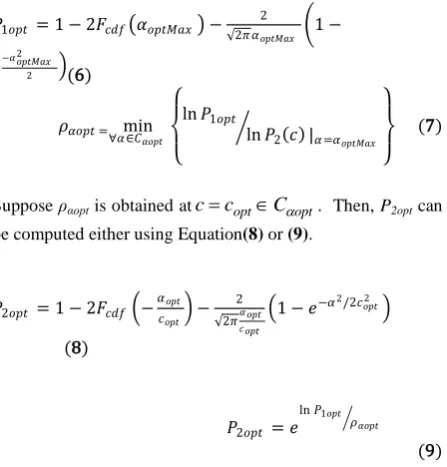
(14) Figure6 shows the computational complexity saving of the proposed optimal load factor over the existing one.
Figure6: Computational complexity saving forα=5 over α=4
From Figure6, for just a million data points (i.e. 𝑛 = 106) 0
5 10 15 20 25 30 35
1 2 3 4 5 6 7 8 9 10
k
n
α = 4 α = 5
x 106
0 200 400 600 800
1 2 3 4 5 6 7 8 9 10
L
n
α = 4 α = 5
x 106
0 25 50 75 100 125 150 175 200
1 2 3 4 5 6 7 8 9 10
Co
m
p
u
tatio
n
al
Co
m
p
lex
it
y
n
α = 4 α = 5
x 106
x 109
0 25 50 75 100
1 2 3 4 5 6 7 8 9 10
CCS
(%
)
there is approximately 75% less computations for using 𝛼 = 5 compared to using𝛼 = 4.
4.2
Memory Requirement
This is the memory space required to store the n data points themselves along with their respective hash values. To store each data point (i.e. 𝒑 ∈ ℜ𝑑) along with its k concatenated hash values on all L tables requires 𝐿(𝑑 + 𝑘) memory. If the k-concatenated values are hashed to produce a single integer, then the memory requirement reduces to 𝐿(𝑑 + 1) per data point. For all n data points, the memory requirement becomes
𝑂(𝑑𝑛𝐿 + 𝑛𝐿). For a large data set this can be huge. In our implementation however, two optimization techniques are used to reduce the memory requirement further. First, all the n data points in
P
are indexed from 1 through n. The indexing is the same across all the L hash tables. This means that each data point is stored once instead of L times. This reduces the memory to 𝑂(𝑑𝑛 + 𝑛𝐿). Second, the single integer produced from hashing the k-concatenated values is not stored but rather used to point to a bucket. The index of the data point is then stored in that bucket. Thus, each data point can be referred to by an index. The hidden constant in𝑂(𝑑𝑛) depends on the data type of the data points in the dataset. Henceforth, the memory analysis concentrates on the hash tables of the data structure. Thus the memory requirement to store the hash tables for all the n data point becomes 𝑂(𝑛𝐿). Once again, L has to be kept at its best minimum to achieve the best memory space. The hidden constant in 𝑂(𝑛𝐿) is the number of bytes required to point to each bucket and 0.125 log2𝑛 bytes to store each index of the data point on each table. For example, for a billion data points (𝑖. 𝑒. 𝑛 ≈ 230) the hidden constant becomes eight bytes. Table 3 shows the memory requirement for using the existing optimal load factor and our proposed optimal load factor.
Table 3. Memory requirements for α = 4 and α = 5 α Memory Requirement
4 𝑂 𝑛1.3508ln 1/𝛿
5 𝑂 𝑛1.2588ln 1/𝛿
The memory requirementsgrow with n. No graph is provided since the expressions on Table 3 are similar to those obtained in Table 2. It is however worth mentioning that he memory saving denoted as MS, for using 𝛼 = 5over𝛼 = 4can be approximatedby Equation (15).
MS ≈ 1 −n10.1 ∗ 100%
(15) From Equation (15), for just a million data points (i.e.
𝑛 = 106) the memory saving for using𝛼 = 5instead of𝛼 = 4isapproximately 75% and this increases as n increases.
4.3
Query Runtime
When running a query 𝒒, two time complexities are involved. First, the time required to hash the query to a bucket on each of the L tables to retrieve the candidate set. Second, the time required to compute the distance between the query and the entries in the candidate set. Let 𝜏 and 𝜏𝑐 denote these
respectively. Computing the hash value 𝑗(𝒑 ) for all the
tables is 𝑂(𝑘𝐿). The second level hash value computation is
𝑂(𝐿) and it is relatively insignificant compared to that of the first. Thus, 𝜏is 𝑂(𝑘𝐿). Suppose it takes one computational
operation to compute the l2 norm between 𝒒 and an entry in
the candidate set. The expected number of entries in the candidate set is 𝛼𝐿. Thus, 𝜏𝑐becomes𝑂(𝛼𝐿). As a result, the total query runtime is 𝑂(𝑘𝐿 + 𝛼𝐿).
If the (𝑅, 𝑐)-NNs are to be sorted then, the computed l2 norms
have to be sorted using a sorting algorithm such as a quick sort. Let this be denoted by𝜏𝑠. The quick sort average computational complexityis 𝑂(𝛼𝐿 log2𝛼𝐿). Thus, the total query runtime becomes τh+τc+τs. The hidden constants in these analyses depend on the dimensionality and the complexity of the data points.
Neglecting the complexities due to computing the distances between the query point and the items in the retrieved buckets and neglecting the complexity due to sorting these distances, the query time complexity is dependent only on the table lookup. Thus, the query time complexity becomes O(𝑛𝜌ln 1/
𝛿 ln n) with a hidden constant factor of −𝜌/ ln 𝑃1 (usually
less than 2).The theoretical query runtime gain, G for using𝛼 = 5over𝛼 = 4canthen be approximated by Equation(16).
𝐺 ≈ 𝑛0.1 (16)
The G, is the ratio of the query runtime for using𝛼 = 5to that of using𝛼 = 4. From Equation (16),for just a million data points (i.e.𝑛 = 106), the query runtime gain for 𝛼 = 5is approximatelyfour times relative to𝛼 = 4.
5.
PRACTICALLSH
IMPLEMENTATION
We present a real-world problem and solve it using LSH parameterization based on existing optimal load factor of
𝛼 = 4and our proposed optimal load factor,𝛼 = 5. It must be emphatically stated that the performance of the LSH algorithm is not dependent on the dataset used. This was evident in all the comparative analyses thathave been conducted in the previous sections. This experiment is to onlyprovide a sample test of the LSH under the proposed load factor compared to the existing load factor. Consequently, there is no need to test the new parameterization of the LSH with several datasets in order to justify that LSH using the proposed load factor always outperforms that of the existing load factor.
5.1
Dataset
The algorithm is tested on real texture features extracted from Defense Meteorological Satellite Program (DMSP) satellite images. The DMSP began in 1991. The visible and infrared sensors collect images across a 3000 km swath, providing global coverage twice per day. Currently, the National Geophysical Data Center (NGDC) receives and processes approximately 8.5 GB of satellite imagery data per day from four DMSP satellites. Each image is downsized to363 x 293.The texture featuresare extracted for 1.6 million images. The dimension for each texture feature vector is
1 x 10 (i.e. 𝑑 = 10) and consists floating point numbers. These features are based on normalized central moments of wavelet edges after multi-resolution decomposition of each image. A detailed discussion of the texture feature extraction approach could be found in[42].
into their scientific predictive models to make real-time predictions such as when and where a hurricane may strike.
5.2
Parameterization
[image:7.595.51.285.194.232.2]Table 4 lists the input parameters and their computed values required to build the hash tables for the dataset using the traditional optimal load factor of 𝛼 = 4 and our proposed optimal load factor of 𝛼 = 5.
Table 4 Corresponding inputs to existing load factor and proposed load factor for n = 1.6 x 10⁶
Inputs α c ρ m k L Existing 4 2.5 0.3508 400009 23 383 Proposed 5 3.3 0.2588 320009 22 105
On Table 4, m is the size of each hash table. That is the number of buckets on each table and this is computed as a prime approximation of 𝑛/𝛼 . The ceiling operator • must be applied to both k and L since both have to be positive integers ( 𝑘, 𝐿 ∈ 𝑍+).
5.3
Hash Table Creation
Below are the steps for building the hash tables for the n data points in the dataset. The creation of the hash tables takes time. As a result, they are created only once and stored along with their families of hash functions. The tables are then used to answer different queries in sublinearqueryruntime.
(1) Generate L families of hash functions, 1, 2, … , 𝐿 randomly and independently from 𝒩(0, 1) such that each 𝑗 = [𝒉𝟏𝒋, 𝒉𝟐𝒋, … , 𝒉𝒌𝒋] and each hash function, 𝒉𝒊𝒋∈ ℜ𝑑∀ 𝑗 ∈ [1, 2, … , 𝐿] and ∀ 𝑖 ∈ [1, 2, … , 𝑘]
(2) Generate an offset, bij randomly, independently and
uniformly from [0, 𝛼] for each ith hash function in each jth family
(3) Generate L set, 𝐻1, 𝐻2, … , 𝐻𝐿 of random integers from the range [1 𝑚], independently such that each 𝐻𝑗 ∈ ℜ𝑘
(4) Index all the n data points in P from 1 through n (5) For each feature vector 𝒑 ∈P, normalized 𝒑 as
𝒑 = 𝒑/ 𝒑 2
(6) Compute the hash value for 𝒑 for the jth family as
𝑗 𝒑 = 𝒉𝟏𝒋•𝒑 +𝑏1𝑗
𝛼 , 𝒉𝟐𝒋•𝒑 +𝑏2𝑗
𝛼 , … , 𝒉𝒌𝒋•𝒑 +𝑏𝑘𝑗
𝛼
(7) Compute the second level hash value for the 𝒑 as
𝑗∗ 𝒑 = (𝑗 𝒑 • 𝐻𝑗)mod 𝑀 mod 𝑚
(8) Store the index of 𝒑 in the bucket 𝑗∗ 𝒑 on the jth table
The M is a large prime integer close to 2𝑊 where, W is the word width of the microprocessor being used. For a 64-bit computer, 𝑀 = 264− 5. In [43, 44],we offered more details regarding the formulation of the equation for computing the hash values.
5.4
Bucket Hashing
Below are the steps to find the (𝑅, 𝑐)-NNs to a query point. (1) For a given query feature vector, 𝒒 ∈P normalized
𝒒(i.e. 𝒒 = 𝒒/ 𝒒 2)
(2) Compute the hash values for 𝒒 as
1 𝒒 , 2 𝒒 , … , 𝐿 𝒒
(3) Compute the second level hash values as
1∗ 𝒒 , 2∗ 𝒒 , … , 𝐿∗ 𝒒
(4) Use the indices in these buckets to collect their corresponding feature vectors (let us call this the candidate set)
(5) Compute the l2 norm between 𝒒 and the entries in the
candidate set
(6) Retrieve the top K, (𝑅, 𝑐)-NNs to 𝒒 or terminate the search once 2𝐿 (including duplicates) items are retrieved
In our implementation, the number of nearest neighbors to be found closest to 𝒒is 𝐾 = 50 (must be less than 2L). The choice of R is better controlled if the data points are normalized. In the l2 normalized space, the l2 norm between
any two data points, 𝒑 and 𝒒 can be computed using Equation (17)
𝒑 − 𝒒 2= 2(1 − 𝒑 • 𝒒 ) (17)
From Equation (17),0 ≤ 𝒑 − 𝒒 2≤ 2. Let λ be the fraction
of the maximum distance within which each (𝑅, 𝑐)-NNs must lie. This means that
cR
is bounded below by 2λ. Consequently, the upper bound of R can be computed as in Equation (18) for any approximation factor, c.𝑅 =2λ𝑐 (18)
It should be noted that if λ is large, the search domain becomes bigger. On the other hand, if λ is too small, the search domain becomes small and only few nearest neighbors could be found. For a highly sparse dataset, λ has to be kept relatively high while for highly dense dataset, λ has to be kept relatively small. We keep λ at 5% (retrieved data points are within 95 percentile of the maximum distance). Thus R becomes 0.0303 units.
5.5
Result and Discussion
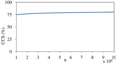
[image:7.595.314.543.629.676.2]Two sets of hash tables are createdusing a 64-bit Intel (R) core (TM) 880 i7 CPU at 3.07/3.20 GHz with 16 GB RAM. The firstset has383 hash tables, each having 400009buckets. This set corresponds to𝛼 = 4.The second set which corresponds to𝛼 = 5, has105 hash tables, each having 320009 buckets. The two sets of hash tables are stored together with their respective families of hash functions. Table 5 summarizes the computational complexities and the memory requirements of the two sets of hash tables.
Table 5 The computational complexities (CC) and memory requirements (MR) for α = 4 and α = 5
α CC (s) CCS (%) MR (MB)
MS (%)
4 13676 - 3092 -
5 3740 73 606 80
From Table 5, under the proposed load factor of
5
, the hash tables are created in much smaller time compared to the time taken to create the hash tables under the existing load factor of𝛼 = 4.In other words, there is 73% less computations to create the hash tables using𝛼 = 5compared to using𝛼 =correctly. In fact, our proposed choice of𝛼 = 5reduces the L to more than a third compared to that of𝛼 = 4(see Table 4). In addition, the memory required to store the hash tables is much smaller under the proposed load factor. To store the hash tables, approximately 80% memory space is saved for using𝛼 = 5 compared to using𝛼 = 4.The theoretical CCS and MS are approximately 75% each (see Equations 15 and 16). Once the tables are created and stored, they can be used to answer queries. Since the data points are indexed, a query is simply referred to by its index. The two sets of hash tables are presented with same ten queries chosen randomly from the dataset and the goal is to report the top 50(𝑅, 𝑐)-NNs to each. Each query is run through a Linear Search (LS) to find the top 50 exact NNs („gold standard‟). Two comparisons are made. First, the 50(𝑅, 𝑐)-NNs for each query reported by each choice for 𝛼 are compared to that of the LS to compute the retrieval percentage accuracy. Second, the query runtimes (𝜏𝐿𝑆𝐻4 and 𝜏𝐿𝑆𝐻5 for 𝛼 = 4 and 𝛼 = 5 respectively) are
compared to the query runtime (𝜏𝐿𝑆) of the LS.These ratios are denoted as G4 and G5 (gains). 𝐺4= 𝜏𝐿𝑆𝐻4/𝜏𝐿𝑆and𝐺5= 𝜏𝐿𝑆𝐻5/𝜏𝐿𝑆for 𝛼 = 4 and 𝛼 = 5 respectively. The query runtime gain of using 𝛼 = 5over 𝛼 = 4 is given by 𝐺 =
𝜏𝐿𝑆𝐻4/𝜏𝐿𝑆𝐻5. The sizes of the candidate sets are expressed as fraction of the number of data points, n and are denoted by CSs4 and CSs5 respectively.
Table6 summarizes these results for the ten queries, which are represented by their indices.
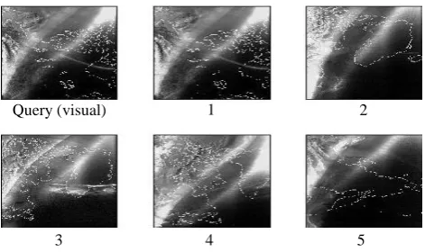
For visual purposes, Figure 7 and Figure 8 show one sample query image (the 970997th image) and its top five similar
[image:8.595.316.552.69.209.2]visual and thermal images respectively. The images are ranked; „1‟ being the best similar image and „5‟ being the worst similar image found respectively.
Figure 7: Visual query image and its top five matches
Figure 8: Thermal query image and its top five matches
Table6.Summarized results for ten random queries reference by their indices
Query index
Retrieval Accuracy (%) Query Runtime (ms) Gain Candidate Set size (%)
4
5
LS
LSH4
LSH5 G4 G5 G CSs4 CSs5412014 100 100 2824.30 52.87 27.10 53 104 2.0 0.28 0.41
497945 100 100 2600.94 26.88 12.69 97 205 2.1 0.28 0.25
783624 100 100 2678.10 35.34 12.17 76 220 2.9 0.28 0.28
970997 100 100 2558.26 37.87 10.82 68 236 3.5 0.27 0.23
1011775 100 100 2677.33 20.16 11.35 133 236 1.8 0.18 0.22
1084917 100 100 2767.25 26.04 16.33 106 169 1.6 0.35 0.38
1191509 100 100 2727.99 19.52 12.29 140 222 1.6 0.19 0.27
1211521 100 100 2653.87 27.85 16.36 95 162 1.7 0.32 0.4
1285384 100 100 3121.96 27.99 20.54 112 152 1.4 0.33 0.57
1507281 100 100 2621.44 23.07 14.55 114 180 1.6 0.25 0.36
Average 100 100 2723.14 29.76 15.42 99 189 2.1 0.27 0.34
From Table 6 the average query runtime gain of using 𝛼 = 5 over using 𝛼 = 4 is approximately 2.It should be noted that both schemes reported the top 50 NNs correctly compared to those reported by the LS. These similar images are same as those reported by the LS.
For the results shown in Figure 7 and Figure 8, the LSH scheme corresponding to 𝛼 = 5 searched only 0.23% whiles that corresponding to 𝛼 = 4searched0.27% of the dataset. Usually we expect 𝐶𝑆𝑠5< 𝐶𝑆𝑠4 but this is not necessarily the case
because the candidate set is the union of the entries in all the buckets collected. If the union operator is not applied then indeed CSs5 would always be less than CSs4.
6.
CONCLUSION
In a large dataset retrieval application in which an approximate match is as good and acceptable as an exact match, LSH is very effective. Unlike the LS, hash tables need to be created when using LSH and this takes time. But once this is done and stored,the benefit of the LSH outweighs that of LS in terms of the query runtime complexity. The goal of the LSH is to search a fraction of the dataset to find the(𝑅, 𝑐)-NNs for any given query data point.This makes LSH scalable for searching large dataset. The number of tables created and the number of projections used have a significant effect on the performance of the LSH. We have shown both theoretically and practically that for𝛼 = 5, the LSH achieves lower computational complexity, lower memory requirement and faster query runtime than usingthe traditional
Query (thermal) 1 2
3 4 5
Query (visual) 1 2
[image:8.595.314.552.246.390.2]optimal load factor of 𝛼 = 4. We therefore propose the use of𝛼 = 5 as an optimal load factor under the LSH scheme. The parameterization discussed based on the l2norm is
extendable to all fractional norms as well. In general, LSH is not effective for small dataset.
7.
ACKNOWLEDGEMENT
This work is partly supported by the Expeditions in Computing by the National Science Foundation (NSF) under Award CCF-1029731 and by National Oceanic and Atmospheric Administration/National Geophysical Data Center (NOAA/NGDC) Educational Program under Cooperative Agreement No: NA060AR4810187. We are very grateful to NSF and NOAA/NGDC.
8.
REFERENCES
[1] Arya, S., Mount, D. M., Netanyahu, N. S., Silverman, R., and Wu, A. Y. 1998. “An optimal algorithm for approximate nearest neighbor searching fixed dimensions,” J. ACM, vol. 45, no. 6, pp. 891-923, 1998).
[2] Flickner, M., Sawhney, H., Niblack, W., Ashley, J., Qian, H., Dom, B., Gorkani, M., Hafner, J., Lee, D., Petkovic, D., Steele, D., and Yanker, P. 1995. “Query by image and video content: the QBIC system,” Computer, vol. 28, no. 9, pp. 23-32, 1995).
[3] Fayyad, U. M. 1996. Advances in knowledge discovery and data mining: AAAI Press.
[4] Lin, K. I., Jagadish, H. V., and Faloutsos, C. 1994. “The TV-tree: an index structure for high-dimensional data,” The VLDB Journal, vol. 3, no. 4, pp. 517-542, 1994).
[5] Roussopoulos, N., Kelley, S., and Vincent, F. 1995. “Nearest neighbor queries,” in Proceedings of the 1995 ACM SIGMOD international conference on Management of data, San Jose, California, United States, pp. 71-79. [6] White, D. A., and Jain, R. "Similarity indexing with the
SS-tree," Data Engineering, 1996. Proceedings of the Twelfth International Conference on. pp. 516-523.
[7] Berchtold, S., Keim, D. A., and Kriegel, H.-P. 1996. “The X-tree: An Index Structure for High-Dimensional Data,” in Proceedings of the 22th International Conference on Very Large Data Bases, pp. 28-39.
[8] Berchtold, S., Böhm, C., Keim, D. A., and Kriegel, H.-P. 1997. “A cost model for nearest neighbor search in high-dimensional data space,” in Proceedings of the sixteenth ACM SIGACT-SIGMOD-SIGART symposium on Principles of database systems, Tucson, Arizona, United States, pp. 78-86.
[9] Cleary, J. G. 1979. “Analysis of an Algorithm for Finding Nearest Neighbors in Euclidean Space,” ACM Trans. Math. Softw., vol. 5, no. 2, pp. 183-192, 1979).
[10] Bentley, J. L., Weide, B. W., and Yao, A. C. 1980. “Optimal Expected-Time Algorithms for Closest Point Problems,” ACM Trans. Math. Softw., vol. 6, no. 4, pp. 563-580, 1980).
[11] Friedman, J. H., Bentley, J. L., and Finkel, R. A. 1977. “An Algorithm for Finding Best Matches in Logarithmic Expected Time,” ACM Trans. Math. Softw., vol. 3, no. 3, pp. 209-226, 1977).
[12] Sproull, R. 1991. “Refinements to nearest-neighbor searching in k -dimensional trees,” Algorithmica, vol. 6, no.
1, pp. 579-589, 1991).
[13] Arya, S., and Mount, D. M. 1995. “Approximate range searching,” in Proceedings of the eleventh annual symposium on Computational geometry, Vancouver, British Columbia, Canada, pp. 172-181.
[14] Preparata, F. P., and Shamos, M. I. 1985. Computational Geometry: An Introduction: Springer-Verlag.
[15] Edelsbrunner, H. 2004. Algorithms in Combinatorial Geometry: Springer.
[16] de Berg, M., Cheong, O., van Kreveld, M., and Overmars, M. 2008. Computational Geometry: Algorithms and Applications: Springer.
[17] Yao, A. C., and Yao, F. F. 1985. “A general approach to d-dimensional geometric queries,” in Proceedings of the seventeenth annual ACM symposium on Theory of computing, Providence, Rhode Island, United States, pp. 163-168.
[18] Clarkson, K. L. 1988. “A randomized algorithm for closest-point queries,” SIAM J. Comput., vol. 17, no. 4, pp. 830-847, 1988).
[19] Agarwal, P. K., and Matoušek, J. 1993. “Ray shooting and parametric search,” SIAM J. Comput., vol. 22, no. 4, pp. 794-806, 1993).
[20] Meiser, S. 1993. “Point location in arrangements of hyperplanes,” Inf. Comput., vol. 106, no. 2, pp. 286-303, 1993).
[21] Gionis, A., Indyk, P., and Motwani, R. 1999. “Similarity Search in High Dimensions via Hashing,” in Proceedings of the 25th International Conference on Very Large Data Bases, pp. 518-529.
[22] Weber, R., Schek, H. J., and Blott, S. 1998. “A Quantitative Analysis and Performance Study for Similarity-Search Methods in High-Dimensional Spaces,” in Proceedings of the 24rd International Conference on Very Large Data Bases, pp. 194-205.
[23] Arya, S., Mount, D. M., Netanyahu, N. S., Silverman, R., and Wu, A. 1994. “An optimal algorithm for approximate nearest neighbor searching,” in Proceedings of the fifth annual ACM-SIAM symposium on Discrete algorithms, Arlington, Virginia, United States, pp. 573-582.
[24] Har-Peled, S. "A Replacement for Voronoi Diagrams of Near Linear Size," 42nd IEEE symposium on Foundations of Computer Science. pp. 94-94.
[25] Indyk, P., and Motwani, R. 1998. “Approximate nearest neighbors: towards removing the curse of dimensionality,” in Proceedings of the thirtieth annual ACM symposium on Theory of computing, Dallas, Texas, United States, pp. 604-613.
[26] Kleinberg, J. M. 1997. “Two algorithms for nearest-neighbor search in high dimensions,” in Proceedings of the twenty-ninth annual ACM symposium on Theory of computing, El Paso, Texas, United States, pp. 599-608. [27] Kushilevitz, E., Ostrovsky, R., and Rabani, Y. 1998.
“Efficient search for approximate nearest neighbor in high dimensional spaces,” in Proceedings of the thirtieth annual ACM symposium on Theory of computing, Dallas, Texas, United States, pp. 614-623.
1999. “When Is ''Nearest Neighbor'' Meaningful?,” in Proceedings of the 7th International Conference on Database Theory, pp. 217-235.
[29] Hinneburg, A., Aggarwal, C. C., and Keim, D. A. 2000. “What Is the Nearest Neighbor in High Dimensional Spaces?,” in Proceedings of the 26th International Conference on Very Large Data Bases, pp. 506-515. [30] Datar, M., Immorlica, N., Indyk, P., and Mirrokni, V. S.
2004. “Locality-sensitive hashing scheme based on p-stable distributions,” in Proceedings of the twentieth annual symposium on Computational geometry, Brooklyn, New York, USA, pp. 253-262.
[31] Andoni, A., and Indyk, P. 2006. “Near-Optimal Hashing Algorithms for Approximate Nearest Neighbor in High Dimensions,” in Proceedings of the 47th Annual IEEE Symposium on Foundations of Computer Science, pp. 459-468.
[32] Slaney, M., and Casey, M. 2008. “Locality-Sensitive Hashing for Finding Nearest Neighbors [Lecture Notes],” Signal Processing Magazine, IEEE, vol. 25, no. 2, pp. 128-131, 2008).
[33] Cormen, T. H., Leiserson, C. E., Rivest, R. L., and Stein, C. 2001. Introduction to Algorithms, Second Edition, p.^pp. 224 -252: MIT Press.
[34] Nolan, J. 2007. Stable Distributions: Models for Heavy-Tailed Data: Springer Verlag.
[35] Buhler, J. 2001. “Efficient large-scale sequence comparison by locality-sensitive hashing,” Bioinformatics, vol. 17, no. 5, pp. 419-428, 2001).
[36] Buhler, J. 2002. “Provably sensitive Indexing strategies for biosequence similarity search,” in Proceedings of the sixth annual international conference on Computational biology, Washington, DC, USA, pp. 90-99.
[37] Buhler, J., and Tompa, M. 2002. “Finding motifs using random projections,” J Comput Biol, vol. 9, no. 2, pp. 225-242, 2002).
[38] Ouyang, Z., Memon, N. D., Suel, T., and Trendafilov, D. 2002. “Cluster-Based Delta Compression of a Collection of Files,” in Proceedings of the 3rd International Conference on Web Information Systems Engineering, pp. 257-268. [39] Shivakumar, N. 1999. “Detecting digital copyright
violations on the internet,” Stanford University.
[40] Cheng, Y. "MACS: music audio characteristic sequence indexing for similarity retrieval," Applications of Signal Processing to Audio and Acoustics, 2001 IEEE Workshop on the. pp. 123-126.
[41] Zolotarev, V. M. 1986. One-Dimensional Stable Distributions: American Mathematical Society.
[42] Gebril, M., Buaba, R., Homaifar, A., and Kihn, E. "Structural indexing of satellite images using automatic classification," Aerospace Conference, 2011 IEEE. pp. 1-7. [43] Buaba, R., Homaifar, A., Gebril, M., and Kihn, E. "Satellite
image retrieval application using Locality Sensitive Hashing in L2-space," Aerospace Conference, 2011 IEEE.
pp. 1-7.