Munich Personal RePEc Archive
The Maastricht convergence criteria and
optimal monetary policy for the EMU
accession countries
Lipinska, Anna
Centre for Economic Performance, LSE
November 2006
Online at
https://mpra.ub.uni-muenchen.de/1795/
The Maastricht convergence criteria and optimal monetary
policy for the EMU accession countries
Anna Lipi´nska
yNovember 2006
Abstract
The EMU accession countries are obliged to ful…ll the Maastricht convergence criteria prior to entering the EMU. What should be the optimal monetary policy satisfying these criteria? To answer this question, the paper proposes a DSGE model of a two-sector small open economy.
First, I derive the micro founded loss function that represents the objective function of the optimal monetary policy not constrained to satisfy the criteria. I …nd that the optimal monetary policy should not only target in‡ation rates in the domestic sectors and aggregate output ‡uctu-ations but also domestic and international terms of trade. Second, I show how the loss function changes when the monetary policy is constrained to satisfy the Maastricht criteria. The loss func-tion of such a constrained policy is characterized by addifunc-tional elements penalizing ‡uctuafunc-tions of the CPI in‡ation rate, the nominal interest rate and the nominal exchange rate around the new targets which are di¤erent from the steady state of the unconstrained optimal monetary policy.
Under the chosen parameterization, the optimal monetary policy violates two criteria: con-cerning the CPI in‡ation rate and the nominal interest rate. The constrained optimal policy is characterized by a de‡ationary bias. This results in targeting the CPI in‡ation rate and the nominal interest rate that are 0.7% lower (in annual terms) than the CPI in‡ation rate and the nominal interest rate in the countries taken as a reference. Such a policy leads to additional welfare costs amounting to 30% of the optimal monetary policy loss.
JEL Classi…cation: F41, E52, E58, E61.
Keywords: Optimal monetary policy, Maastricht convergence criteria, EMU accession coun-tries
I would like to thank Kosuke Aoki for his excellent supervision and encouragement. I also thank Evi Pappa, Hugo Rodriguez, Gianluca Benigno and Michael Woodford for helpful comments and suggestions. Part of this work was done while I was visiting the European Central Bank. I would like to thank the members of the Monetary Policy Strategy Division for valuable discussions and hospitality.
yInternational Doctorate in Economics Analysis, Universitat Autònoma de Barcelona, Edi…ci B - Campus de la
1
Introduction
On May 1, 2004 eight countries from Central and Eastern Europe (i.e. Czech Republic, Estonia, Hungary, Latvia, Lithuania, Poland, Slovakia and Slovenia) together with Cyprus and Malta entered the European Union (EU). Importantly, the Accession Treaty signed by all these countries includes an obligation to participate in the third stage of the economic and monetary union, i.e. an obligation to enter the European Monetary Union (EMU) in the near future. Moreover, in order to enter the EMU, these countries are required to satisfy the Maastricht convergence criteria (Treaty of Maastricht, Article 109j(1)). The criteria are designed to guarantee that prior to joining the European Monetary Union, countries attain a high degree of economic convergence not only in real but also in nominal terms. To this end, the Article 109j(1) of the Maastricht Treaty lays down the following criteria as a prerequisite for entering the EMU:1
the achievement of a high degree of price stability which means that a Member State (of the
EU) has a sustainable price performance and an average rate of in‡ation (the Consumer Price Index (CPI) in‡ation), observed over a period of one year before the examination, which does not exceed that of the three best performing Member States in terms of price stability by more than 1.5% points (the CPI in‡ation rate criterion);
the durability of the convergence ... re‡ected in the long term interest rate levels which means
that, over a period of one year before the examination, a Member State has an average nominal long-term interest rate that does not exceed that of the three best performing Member States in terms of price stability by more than 2% points (the nominal interest rate criterion);
the observance of the normal ‡uctuation margins provided for by the Exchange Rate Mechanism
of the European Monetary System( 15%bound around the central parity), for at least two years,
without devaluing against the currency of any other Member State (the nominal exchange rate criterion).
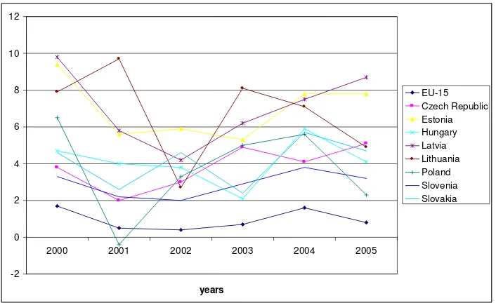
By setting constraints on the monetary variables, these criteria a¤ect the way monetary policy should be conducted in the EMU accession countries. Importantly, monetary policy plays a crucial role in the stabilization process of an economy exposed to shocks. The stochastic environment of the EMU accession countries has both domestic and external origins. As far as the domestic environment is concerned, a strong productivity growth has been observed in the EMU accession countries in the last years (see Figure 1 in Appendix A). Moreover, all these countries are small open economies which also makes them vulnerable to external shocks (see Table 1 in Appendix A).
1Importantly, the Maastricht Treaty also imposes the criterion on the …scal policy, i.e. the sustainability of the
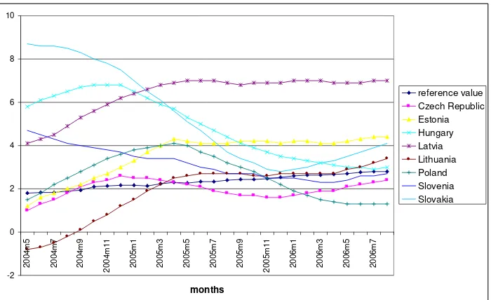
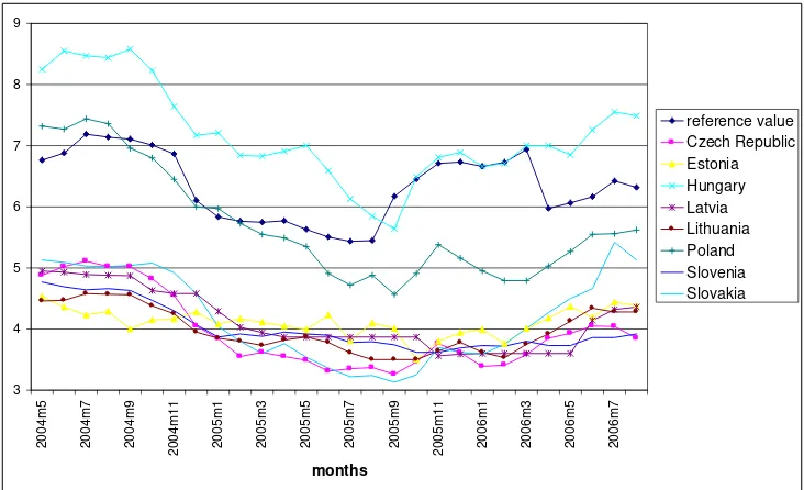
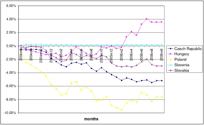
An obligation to ful…ll the Maastricht convergence criteria by the EMU accession countries can restrict the stabilization role of the monetary policy. At the moment, many EMU accession countries do not satisfy some of the Maastricht convergence criteria. Estonia, Hungary, Latvia, Lithuania and Slovakia fail to ful…ll the CPI in‡ation rate criterion (see Figures 2 and 3 in Appendix A). Moreover, Hungary also violates the nominal interest rate criterion (see Figures 4 and 5 in Appendix A). On the other hand, the nominal exchange rate ‡uctuations versus the euro for all EMU accession countries remain within the band set by the nominal exchange rate criterion (see Figure 6 in Appendix A).
Keeping this in mind, two natural questions arise. Are the Maastricht convergence criteria compat-ible with the optimal monetary policy in the EMU accession countries? What are the characteristics of the optimal policy that satis…es the Maastricht convergence criteria? The goal of this paper is to answer these questions. To this purpose, we develop a DSGE model of a small open economy with nominal rigidities exposed to both domestic and external shocks.
The production structure of the economy is composed of two sectors: a nontraded good sector and a traded good sector. There are several reasons why we decide to impose such a structure in our model. According to the literature, the existence of the nontraded sector helps us explain international business cycle ‡uctuations and especially real exchange rate movements (e.g. Benigno and Thoenisen (2003), Corsetti et al. (2003), Stockman and Tesar (1994)). Moreover, the empirical studies regarding the OECD countries …nd that a major part of the aggregate ‡uctuations rather have their source in sector-speci…c than country-wide shocks (e.g. Canzoneri et al. (1999), Marimon and Zilibotti (1998)). Finally, we want to match our model with the empirical literature on the EMU accession countries that emphasizes the role of sector productivity shocks in shaping in‡ation and real exchange rate patterns in these countries (e.g. Mihaljek and Klau (2004)).
In this framework, we characterize the optimal monetary policy from a timeless perspective (Wood-ford (2003)). We derive the micro founded loss function using the second-order approximation method-ology developed by Rotemberg and Woodford (1997) and Benigno and Woodford (2005). We …nd that the optimal monetary policy (unconstrained policy) should not only target in‡ation rates in the do-mestic sectors and aggregate output ‡uctuations, but also dodo-mestic and international terms of trade. Since the Maastricht convergence criteria are not easily implementable in our model, we reformulate them using the methodology developed by Rotemberg and Woodford (1997, 1999) for the analysis of the zero bound problem of the nominal interest rate. This method enables us to verify whether a given criterion is satis…ed by only computing …rst and second moments of a variable for which the criterion is set. We focus on the criteria imposed on the CPI in‡ation rate, the nominal interest rate and the nominal exchange rate as we do not explicitly model the …scal policy. Moreover, we present how the loss function changes when the monetary policy is constrained by the Maastricht convergence crite-ria. Finally, we derive the optimal monetary policy that satis…es all Maastricht convergence criteria (constrained policy).
rate and the nominal interest rate. The optimal policy which satis…es these two criteria also guarantees satisfaction of the nominal exchange criterion. Both the stabilization component and the determin-istic component of the constrained policy are di¤erent from the unconstrained optimal policy. The constrained policy leads to a smaller variability of the CPI in‡ation, the nominal interest rate and the nominal exchange rate than under optimal monetary policy. Moreover, it is also characterized by a de‡ationary bias which results in targeting a CPI in‡ation rate and a nominal interest rate that are 0.7% lower (in annual terms) than the CPI in‡ation rate and the nominal interest rate in the reference countries. As a result, the policy constrained by the Maastricht convergence criteria induces addi-tional welfare costs which amount to 30% of the initial deadweight loss associated with the optimal monetary policy.
The literature has so far concentrated on two aspects of monetary policy in the EMU accession countries: the appropriate monetary regime in the light of the future accession to the EMU and also the ability of the alternative monetary regimes to comply with the Maastricht convergence criteria. The …rst stream of literature represented by, among others, Buiter and Grafe (2003), Coricelli (2002), calls for adopting the peg regime to the euro in these countries, as it enhances the credibility of the monetary policy and also strengthens the links with the EU and the EMU. Moreover, using a DSGE model with nominal rigidities and imperfect credibility, Ravenna (2005) …nds that the gain from a credible adoption of the …xed regime towards the euro can outweigh the loss of resignation from the independent monetary policy. Nevertheless, Buiter and Grafe (2003) also claim that an adoption of the …xed regime can seriously endanger the ful…llment of the CPI in‡ation criterion and therefore call for a change in this criterion. Their reasoning is based on the empirical studies regarding sources of the CPI in‡ation and real exchange rate developments in the EMU accession countries. A majority of the studies2 concentrate on the Balassa–Samuelson e¤ect (Balassa (1964)), which predicts that countries experiencing a higher productivity growth in the traded sector are also characterized by a higher CPI in‡ation rate and real exchange rate appreciation. Others (e.g. Mihaljek and Klau (2004)) also highlight the role of productivity shocks in the nontraded sector in a¤ecting the CPI in‡ation rate and the real exchange rate appreciation in the EMU accession countries.3
The second stream of the literature builds an analysis in the framework of open economy DSGE models. Devereux (2003) and Natalucci and Ravenna (2003) …nd that the monetary regime character-ized by ‡exible in‡ation targeting with some weight on exchange rate stability succeeds in ful…lling the Maastricht criteria. Two other studies are also worth noting: Laxton and Pesenti (2003) and Ferreira (2006). The authors of the …rst paper study how di¤erent interest rate rules perform in stabilizing variability of in‡ation and output in a small open economy. The second paper focuses on calculation of the welfare loss that the EMU accession countries will face when they join the EMU. However,
2We can list the following empirical studies that analyze CPI in‡ation and real exchange rate developments in the
EMU accession countries: Cipriani (2001), de Broeck and Slok (2001), Egert et al. (2002), Fisher (2002), Halpern and Wyplosz (2001), Coricelli and Jazbec (2001), Arratibel et al. (2002), Mihaljek and Klau (2004).
3This study goes in line with a recent paper by Altissimo et al (2004) on the sources of in‡ation di¤erentials in the
contrary to our study, it does not provide the micro founded welfare criterion.
In contrast to previous studies, our analysis is characterized by the normative approach. We construct the optimal monetary policy for a small open economy and contrast it with the optimal policy that is also restricted to satisfy the Maastricht convergence criteria. Therefore, our framework enables us to set guidelines on the way in which monetary policy should be conducted in the EMU accession countries.
The rest of the paper is organized as follows. The next section introduces the model and derives the small open economy dynamics. Section 3 describes derivation of the optimal monetary policy. Section 4 presents the way we reformulate the Maastricht convergence criteria in order to implement them in our framework. Section 5 is dedicated to the derivation of the optimal policy constrained by the Maastricht convergence criteria. Section 6 compares the optimal monetary policy with the optimal monetary policy constrained by the Maastricht convergence criteria under the chosen parameterization of the model. Section 7 concludes.
2
The model
Our modelling framework is based on a one-sector small open economy model of de Paoli (2004) where all goods, i.e. home and foreign ones, are tradable. We extend this model by incorporating two domestic sectors, i.e. a nontraded and a traded sector. Our model is also closely related to the studies of Devereux (2003) and Natalucci and Ravenna (2003). However, we relax an assumption present in their studies regarding perfect competition and homogeneity of goods in the traded sector, which enables us to discuss a role of terms of trade in the stabilization process of a small open economy. In that way our modelling framework is similar to a two-country model with two production sectors of Liu and Pappa (2005).
Following de Paoli (2004), we model a small open economy as the limiting case of a two-country problem, i.e. where the size of the small open economy is set to zero. In the general framework, the model represents two economies of unequal size: a small open home economy and a foreign large economy (which is proxied as the euro area). We consider two highly integrated economies where asset markets are complete. In each of the economies, there are two goods sectors: nontraded goods and traded goods. Moreover, we assume that labour is mobile between sectors in each country and immobile between countries. We assume the existence of home bias in consumption which, in turn, depends on the relative size of the economy and its degree of openness. This assumption enables us to consider a limiting case of the zero size of the home economy and concentrate on the small open economy.
economies.4 The stochastic environment of the small open economy is characterized by asymmetric productivity shocks originating in both domestic sectors, preference shocks and foreign consumption shocks.
2.1
Households
The world economy consists of a continuum of agents of unit mass: [0; n)belonging to a small country (home) and[n;1]belonging to the rest of the world, i.e. the euro area (foreign). There are two types of di¤erentiated goods produced in each country: traded and nontraded goods. Home traded goods are indexed on the interval[0; n)and foreign traded goods on the interval[n;1], respectively. The same applies to nontraded goods. In order to simplify the exposition of the model, we explain in detail only the structure and dynamics of the domestic economy. Thus, from now on, we assume the size of the domestic economy to be zero, i.e. n!0.
Households are assumed to live in…nitely and behave according to the permanent income hypoth-esis. They can choose between three types of goods: nontraded, domestic traded and foreign traded goods. Cti represents consumption at periodt of a consumeri andLit constitutes his labour supply. Each agent imaximizes the following utility function:5
maxEt0
( 1
X
t=t0
t t0 U Ci
t; Bt V Lit )
; (1)
whereEt0denotes the expectation conditional on the information set at datet0, is the intertemporal discount factor and0< <1; U( )stands for ‡ows of utility from consumption andV( )represents ‡ows of disutility from supplying labour.6 Cis a composite consumption index. We de…ne consumers’ preferences over the composite consumption indexCtof traded goods (CT;t) (domestically produced and foreign ones) and nontraded goods (CN;t):
Ct 1C 1
N;t + (1 )
1 C
1
T;t 1
; (2)
where >0is the elasticity of substitution between traded and nontraded goods and 2[0;1]is the share of the nontraded goods in overall consumption. Traded good consumption is a composite of the domestically produced traded goods (CH) and foreign produced traded goods (CF):
CT;t h(1 )1C 1
H;t + 1
C 1
F;t i 1
; (3)
4See Woodford (2003).
5In general, we assumeU to be twice di¤erentiable, increasing and concave inC
tandV to be twice di¤erentiable, increasing and convex inLt.
6We assume speci…c functional forms of consumption utilityU Ci
t , and disutility from labourV Lit : U Cti
(Cit)1 Bt
1 ; V L
i t 'l
(Lit)1+
1+ with ( >0), the inverse of the intertemporal elasticity of substitution in consumption
where >0 is the elasticity of substitution between home traded and foreign traded goods, and is the degree of openness of the small open economy ( 2[0;1]).7 Finally,C
j (wherej=N; H; F) are
consumption sub-indices of the continuum of di¤erentiated goods:
Cj;t 2 4 1
n 1 Zn
0
ct(j) 1dj 3 5
1
; (4)
where >1 represents elasticity of substitution between di¤erentiated goods in each of the sectors. Based on the above presented preferences, we derive consumption-based price indices expressed in the units of currency of the domestic country:
Pt h
PN;t1 + (1 )PT;t1 i 1 1
; (5)
PT;t h
PH;t1 + (1 )PF;t1 i 1 1 (6) with Pj;t 2 4 1 n n Z 0
pt(j)1 dj 3 5
1 1
: (7)
Although we assume the law of one price in the traded sector (i.e. p(h) =Sp (h)andp(f) =Sp (f)
where S is the nominal exchange rate), both the existence of the nontraded goods and the assumed home bias cause deviations from purchasing power parity, i.e. P 6=SP . The real exchange rate can be de…ned in the following manner: RS SP
P : Moreover, we de…ne the international terms of trade
asT PF
PH and the ratio of nontraded to traded goods’ prices (domestic terms of trade) asT
d PN
PT:
From consumer preferences, we can derive total demand for the generic goods –n(home nontraded ones),h(home traded ones),f (foreign traded ones):
yd(n) = p(n)
PN
PN
P C; (8)
yd(h) = p(h)
PH
PH
PT (1 )CT+ p (h)
PH
PH
PT CT; (9)
yd(f) = p (f)
PF
PF
PT CT (10)
7Following de Paoli (2004) and Sutherland (2002), we assume home bias ( ) of the domestic households to be a
where variables with an asterisk represent the foreign equivalents of the domestic variables. Impor-tantly, since the domestic economy is a small open economy, demand for foreign traded goods does not depend on domestic demand. However, at the same time, demand for domestic traded goods depends on foreign demand.
Households get disutility from supplying labour to all …rms present in each country. Each individual supplies labour to both sectors, i.e. the traded and the nontraded sector:
Lit=Li;Ht +Li;Nt : (11) We assume that consumers have access to a complete set of securities-contingent claims traded internationally. Each household faces the following budget constraint:
PtCti+EtfQt;t+1Dt+1g Dt+T Rti+WH;ti LiH;t+WN;ti LiN;t+ n R
0
i N;tdi
n +
n R
0
i H;tdi
n ; (12)
where at date t, Dt+1 is nominal payo¤ of the portfolio held at the end of period (t), Qt;t+1 is the
stochastic discount factor for one-period ahead nominal payo¤s relevant to the domestic household,
H;t and N;t are nominal pro…ts from the domestic …rms andT Rti are nominal lump-sum transfers
from the domestic government to householdi. Moreover, consumers face no Ponzi game restriction. The short-term interest rate(Rt)is de…ned as the price of the portfolio which delivers one unit of
currency in each contingency that occurs in the next period:8
Rt1=EtfQt;t+1g: (13)
The maximization problem of any household consists of maximizing the discounted stream of utility (1) subject to the budget constraint (12) in order to determine the optimal path of the consumption index, the labour index and contingent claims at all times. The solution to the household decision problem gives a set of …rst-order conditions.9 Optimization of the portfolio holdings leads to the following Euler equations for the domestic economy:
UC(Ct; Bt) = Et UC(Ct+1; Bt+1)Qt;t1+1
Pt Pt+1
: (14)
There is a perfect sharing in this setting, meaning that marginal rates of consumption in nominal terms are equalized between countries in all states and at all times.10 Subsequently, appropriately choosing the distribution of initial wealth, we obtain the risk sharing condition:
8Following the literature, we assume one period to be one quarter.
9We here suppress subscripti as we assume that in equilibrium, all agents are identical. Therefore, we represent
optimality conditions for a representative agent.
1 0We have to point out here that although the assumption of complete markets conveniently simpli…es the model, it
UC(Ct; Bt) UC(Ct; Bt) =
Pt
StPt = RS
1
t ; (15)
where >0and depends on the initial wealth distribution. The risk sharing condition implies that the real exchange rate is equal to the marginal rate of substitution between domestic and foreign consumption.
The optimality condition for labour supply in the domestic economy is the following:
Wk t Pt =
VL(Lt)
UC(Ct; Bt); (16)
where Wk is the nominal wage of the representative consumer in sectork(k=H; N):11 So the real wage is equal to the marginal rate of substitution between labour and consumption.
2.2
Firms
All …rms are owned by consumers. Both traded and nontraded sectors are monopolistically competi-tive. The production function is linear in labour which is the only input. Consequently, its functional form for …rmiin sectork(k=N; H) is the following:
Yk;t(i) =AktLkt(i): (17) Price is set according to the Calvo (1983) pricing scheme. In each period, a fraction of …rms
(1 k)decides its price, thus maximizing the future expected pro…ts. The maximization problem of
any …rm in sectorkat timet0is given by:
max
Pk;t0(i) Et0
1
X
t=to
( k)sQt0;t (1 k)Pk;t0(i) M C k
t(i) Yk;td 0:t(i)
subject to Yk;td0:t(i) =
Pk;t0(i)
Pk;t Yk;t; (18)
where Yd
k;t0:t(i) is demand for the individual good in sector k produced by producer i at time t conditional on keeping the price Pk;t0(i) …xed at the level chosen at time t0; M C
k t =
Wk t(i) Ak
t is the
nominal marginal cost in sectorkat time t, and k are revenue taxes in sectork.
Given this setup, the price index in sectork evolves according to the following law of motion:
(Pk;t)1 =
k(Pk;t 1)1 + k(Pk;t0(i))
1 : (19)
1 1Notice that wages are equalized between sectors inside each of the economies, due to perfect labour mobility and
2.3
Fiscal and monetary policies
The government in the domestic economy is occupied with collecting revenue taxes from …rms that are later redistributed to households in the form of lump-sum transfers in such a way that each period, there is a balanced budget:
n Z
0
( NPN;t(i)YN;t(i) + HPH;t(i)YH;t(i))di= n Z
0
T Rjtdj: (20)
A role for the monetary policy arises due to existing nominal and real rigidities in the economy: price stickiness (together with monopolistic competition), home bias and the nontraded good sector, which lead to deviations from PPP. The system is therefore closed by de…ning appropriate monetary rule for the domestic economy.
2.4
A loglinearized version of the model
This section presents a system of the equilibrium conditions for the small open economy in the loglinear form, which is derived through the …rst-order approximation around the deterministic steady state with zero in‡ation de…ned in Appendix B. Here, we characterize the dynamic features of this model where the variables with a hat stand for the log deviations from the steady state. Additionally, the variables with an asterisk represent the foreign equivalents of the domestic variables.
The supply-side of the economy is given by two Phillips curves, one for the nontraded and one for the domestic traded sector, respectively, which are derived from (18):
bN;t=kN( Cbt+ Lbt AbN;t Bbt pbN;t) + bN;t+1; (21)
bH;t=kH( Cbt+ Lbt AbH;t Bbt pbH;t) + bH;t+1 (22)
wherebN;t ln(PPN;tN;t1);bH;t ln( PH;t PH;t 1); kN
(1 N)(1 N )
N ;kH
(1 H)(1 H )
H and aggregate
labour supply (Lbt) is de…ned through the labour market clearing condition ((11), (17)):
b
Lt=deYN(YbN;t AbN;t) +deYH(YbH;t AbH;t); (23)
wheredYeN
YN YN+YH;
e dYH
YH
YN+YH are ratios evaluated in the steady state (see Appendix B).
It is worth underlining that in‡ation dynamics in both domestic sectors do not only depend on the real marginal costs in a given sector, but also on the relative prices of goods. In particular, a higher relative price of goods in one sector in relation to other goods induces a substitution away e¤ect and leads to de‡ationary pressures in this sector.
b
YN;t=Cbt pbN;t; (24)
b
YH;t=dCHCtb pH;tb +b( )dCHTbtd+ (1 dCH) RStc +
+ (1 dCH)Cbt +b ( )(1 dCH)Tbtd (25)
where dCH (1 )(1 )C
YHpH pT ; b (pN)
1 ; b (p
N)1 are ratios evaluated in the
steady state (see Appendix B). Additionally, we de…ne aggregate output as the sum of sector outputs:
b
Yt=dY N(bpN;t+YN;tb ) +dY H(pH;tb +YH;tb ); (26) wheredY N pNYYN anddY H pHYYH are ratios evaluated in the steady state (see Appendix B):
The complete asset market assumption (15) gives us the following risk sharing condition:
b
Ct=Btb +1RStc +Cbt Bbt: (27) From the de…nition of price indices ((5), (6)), we obtain the following relations between relative prices, terms of trade, domestic terms of trade and real exchange rate:
(a 1)pH;tb =bTcd
t +aRStd b aTdtd ; (28)
b
pN;t= (1 b)Tctd; (29)
b
pH;t= bTctd aTbt; (30)
where a RSpF pT
1
is the ratio evaluated in the steady state (see Appendix B). We also derive the laws of motion for the international terms of trade and the domestic terms of trade from their de…nitions:
b
Tt=bF;t bH;t+Tbt 1; (31)
b
Ttd=bN;t bT;t+Tbtd1; (32)
wherebT;t= (1 a)bH;t+abF;tandbF;t=bF;t+(Stb Stb 1)withbT;t ln(PPT ;tT ;t1),bF;t ln(PPF;tF;t1), bF;t ln(
PF;t PF;t 1)
:
nominal interest rate (Rtb )and the nominal exchange rate (Stb). First, the nominal interest rate can be derived from the loglinearized version of the Euler condition (14):
b
Rt= (Cbt+1 Bbt+1) (Cbt Bbt) +bt+1; (33)
where bt ln(PPtt1):CPI aggregate in‡ation is a weighted sum of the sector in‡ation rates:
bt=bbN;t+ (1 a)(1 b)bH;t+a(1 b)bF;t+a(1 b)(Sbt Sbt 1): (34)
Notice that CPI aggregate in‡ation does not only depend on the domestic sector in‡ation rates, but also on the foreign traded in‡ation rate and changes in the nominal exchange rate. For example, a nominal exchange rate depreciation puts an upward pressure on the CPI in‡ation rate.
The nominal exchange rate can be derived from the de…nition of the real exchange rate:
b
St=Stb 1+bt bt +RStc RStc 1: (35)
The law of motion of the nominal exchange rate depends on the real exchange rate ‡uctuations and di¤erences in the aggregate in‡ation rates between the home and the foreign economy. Additionally, by combining the international risk sharing condition (27) and Euler conditions for the domestic and foreign economy (33), we obtain a relation between the nominal interest rate and the nominal exchange rate:
b
St=Rbt Rtb +Stb+1: (36)
This equation represents a version of the uncovered interest rate parity, which implies that changes in the nominal exchange rate result from di¤erences between the domestic and foreign monetary policy. Let us point out that although very intuitive, this equation does not constitute an independent equilibrium condition.
The system is closed by specifying a monetary rule. In this paper, we derive the optimal monetary policy rule which maximizes welfare of the society subject to the structural equations of the economy. The optimal rule is speci…ed as a rule where the monetary authority stabilizes the target variables in order to minimize the welfare loss of society and provide the most e¢cient allocation.12 Apart from the optimal monetary derivation in this framework, we also consider the optimal monetary policy which is additionally constrained by the Maastricht convergence criteria.
Summing up, the dynamics of the small open economy are summarized by the following variables,
bN;t;bH;t;Ct;b Lt;b YH;t;b YN;t;b pN;t;b pH;t;b Yt;b RSt;c Tbd
t;Tt;b St;b bt;Rtb which are determined by equations
(21)–(35), given the evolution of the stochastic shocks AbN;t; AbH;t; Bbt and the foreign variablesCbt; b
Td
t ; bt; bF;t:13
1 2Giannoni and Woodford (2003) call these type of rules ‡exible in‡ation targeting rules.
1 3For simplicity, we choose to consider only one type of external shocks, foreign consumption shocks (Cb
3
The optimal monetary policy
This section characterizes the optimal monetary policy, i.e. the policy maximizing welfare of society subject to the structural equations of an economy. The micro foundations of our model give us a natural welfare measure, i.e. a discounted sum of expected utilities for the agents in the economy (see equation (1)).
We use a linear quadratic approach (Rotemberg and Woodford (1997, 1999)) and de…ne the optimal monetary policy problem as a minimization problem of the quadratic loss function subject to the loglinearized structural equations (presented in the previous section). First, we present the welfare measure derived through a second-order Taylor approximation of equation (1):
Wt0 =UCCEt0
1
X
t=t0 t t0[
z0
vbvt
1 2bv
0
tZvbvt vb
0
tZ bt] +tip+O(3); (37)
wherebv0
t= h
b
Ct YbN;t YbH;t bN;t bH;t i
;b0t=h AbN;t AbH;t Bbt Cbt i
;
z0
v = h
1 sCdYeN sCdYeH 0 0 i
and matrices Zv; Z are de…ned in Appendix B; tip
stands forterms independent of policy andO(3)includes terms that are of a higher order than the second in the deviations of variables from their steady state values.
Notice that the welfare measure (37) contains the linear terms in aggregate consumption and sector outputs. These linear terms result from the distortions in the economy. First, monopolistic competition in both domestic sectors leads to ine¢cient levels of sector outputs and subsequently, an ine¢cient level of aggregate output. Second, since the domestic economy is open, domestic consump-tion and aggregate output are not equalized. Importantly, their composiconsump-tion depends on the domestic and international terms of trade. Third, there exists a(n) (international) terms of trade externality (see Corsetti and Pesenti (2001)) according to which monetary policy has an incentive to generate a welfare improving real exchange rate appreciation which leads to a lower disutility from labour without a corresponding decline in the utility of consumption.
The presence of linear terms in the welfare measure (37) means that we cannot determine the optimal monetary policy, even up to …rst order, using the welfare measure subject to the structural equations (21)–(35) that are only accurate to …rst order. Following the method proposed by Benigno and Woodford (2005) and Benigno and Benigno (2005), we substitute the linear terms in the ap-proximated welfare function (37) by second moments of aggregate output, domestic and international terms of trade using a second-order approximation to the structural equations of the economy.14 As a result, we obtain the fully quadratic loss function which can be represented as a function of aggregate output (Ytb), domestic and international terms of trade (Tbd
t; Ttb) and domestic sector in‡ation rates
(bH;t;bN;t). Its general expression is given below:
result,Tbd
t ;bt;bF;t are assumed to be zero. Moreover, all shocks follow an AR(1) process with normally distributed innovations.
Lt0=UCCEt0
1
X
t=t0
t t0[1
2 Y(Ybt Yb
T t )2+
1 2 Td(Tb
d t Tbd
T t )2+
1
2 T(Tbt Tb
T
t )2+ T TdTbtdTbt+ Y TdYbtTbtd+ Y TYbtTbt+
+1 2 Hb
2
H;t+
1 2 Nb
2
N;t] +tip+O(3); (38)
whereYbtT;TbtdT;TbtT are target variables which are functions of the stochastic shocks and, in general, are di¤erent from the ‡exible price equilibrium processes of aggregate output, domestic terms of trade and international terms of trade.15 The coe¢cients
Y; Td; T; T Td; Y Td; Y T; H; N are
functions of the structural parameters of the model. The term tipstands forterms independent of policy.
Our loss function can be seen as a generalization of the previous studies encompassing both the closed (Aoki (2001), Benigno (2004), Rotemberg and Woodford (1997)) and open economy frameworks (Gali and Monacelli (2005), de Paoli (2004)).16 Notice that if we set the size of the nontraded sector to zero and therefore obtain a one-sector small open economy, the loss function becomes identical to the loss function derived by de Paoli (2004).17 In this case, the loss function is a function of the variances of aggregate output, terms of trade18 and home traded in‡ation. On the other hand, if we set the degree of openness to zero, we obtain the case of a two-sector closed economy which was studied by Aoki (2001) and Benigno (2004). Here, the loss function is a function of the variances of aggregate output, domestic terms of trade, the covariance term between the two and variances of the sector in‡ation rates. Additionally, our loss function is closely related to the loss function derived for a national policymaker in a two-country model with two sectors of Liu and Pappa (2005). Interestingly, since their model is absent from the monopolistic competition distortion, trade imbalances and also expenditure switching e¤ect, the loss function of a national policymaker depends only on the sector in‡ation rates and the sector output ‡uctuations around the ‡exible price targets.
We characterize the optimal plan under commitment where the policy maker chooses the set of variables
fbN;t;bH;t;Cbt;Lbt;YbH;t;YbN;t;pbN;t;bpH;t;Ybt;RSct;Tbtd;Tbt;Sbt;bt;Rbtg1t=t0 in order to minimize the loss
1 5As previously shown in papers by Gali and Monacelli (2005) and de Paoli (2004), in the small open economy
framework the target variables will be identical to the ‡exible price allocations only in some special cases, i.e. an e¢cient steady state, no markup shocks, no expenditure switching e¤ect (i.e. = 1) and no trade imbalances.
1 6Rotemberg and Woodford (1998) present a one-sector closed economy model. Aoki (2001) presents a two-sector
closed economy model with sticky prices only in one of the sectors. Benigno (2004) analyses the case of a monetary union comprised of two countries, which can be interpreted as a two-sector closed economy with totally segmented labour markets (interpretation as in Woodford (2003)). Gali and Monacelli (2005) and de Paoli (2004) study the case of a one-sector small open economy.
1 7In our representation, there is a covariance term between terms of trade and aggregate output which can be
represented as the weighted sum of the variances of aggregate output and terms of trade.
1 8In the analysis of de Paoli (2004), it is actually the variance of the real exchange rate. However, it must be kept in
function (38) subject to constraints (21)–(35), given the initial conditions on this set of variables.19 To simplify the exposition of the optimal plan, we reduce the number of variables to the set of …ve domestic variables which determine the loss function (38), i.e. Yt;b Tbd
t;Tt;b bN;t; bH;t. Therefore, we
represent the structural equations of the two-sector small open economy (21)–(35) in terms of these variables. The coe¢cients are de…ned in Appendix B.
The supply side of the economy is represented by two Phillips curves which are derived from equations (21) and (22) through a substitution of aggregate consumption, aggregate labour and relative prices:
bN;t=kN(mN;YYtb +mN;TdTbtd+mN;TTtb +mN;ANAN;tb +
+mN;AHAH;tb +mN;BBtb) + bN;t+1; (39)
bH;t=kH(mH;YYbt+mH;TdTbtd+mH;TTbt+mH;ANAbN;t+
+mH;AHAbH;t+mH;BBbt) + bH;t+1: (40)
The equation describing the demand side of the economy is derived from the market clearing conditions ((24), (25)) and the risk sharing condition (27):
b
Ct =Ytb +nTdTbtd+nTTtb +nBBt;b (41)
where aggregate consumption, relative prices and real exchange rate were substituted out.
The last structural equation represents the law of motion of the domestic and international terms of trade:
b
Ttd Tbtd 1=bN;t bH;t a(Ttb Ttb 1): (42)
Finally, the policy maker following the optimal plan under commitment choosesfYt;b Tbtd;Tt;b bH;t;bN;tg1t=t0 in order to minimize the loss function (38) subject to the constraints (39)–(42), given the initial con-ditions onYbt0;Tb
d
t0;Tbt0;bH;t0;bN;t0. The …rst-order conditions of the problem are the following (where
i;t withi= 1;2;3;4 are accordingly the Lagrange multipliers with respect to (39)– (42)):
with respect to bN;t:
NbN;t+ 1;t 1;t 1 4;t= 0; (43)
1 9The initial conditions guarantee the timeless perspective of the problem and make the …rst-order conditions of the
with respect to bH;t:
HbH;t+ 2;t 2;t 1+ 4;t= 0; (44)
with respect to Ytb :
Y(Ybt YbtT) + Y TdTbtd+ Y TTbt kNmN;Y 1;t kHmH;Y 2;t 3;t= 0; (45)
with respect to Tbd t :
Td(Tbtd Tbd T
t ) + T TdTtb + Y TdYtb kNmN;Td 1;t kHmH;Td 2;t
+nTd 3;t+ 4;t 4;t+1= 0; (46)
with respect to Ttb :
T(Tbt TbtT) + T TdTbtd+ Y TYbt kNmN;T 1;t kHmH;T 2;t
+nT 3;t+a 4;t a 4;t+1= 0: (47)
Equations (43)–(47) and constraints (39)–(42) fully characterize the behaviour of the economy under the optimal monetary policy.
4
The Maastricht convergence criteria – a reinterpretation
Including the Maastricht criteria in their original form as additional constraints of the optimal mon-etary policy requires computationally demanding techniques. In particular, it results in solving the minimization problem of the loss function (38) subject to additional nonlinear constraints. On the other hand, the linear quadratic approach has two important advantages that make us decide to re-formulate the criteria. First, it provides us with the analytical and intuitive expression for the loss function which can also serve as a welfare measure to rank alternative suboptimal policies. Second, the linear quadratic approach makes it easy to check second-order conditions (which would otherwise be quite di¢cult) for local optimality of the derived policy.
Therefore, the purpose of this section is to describe the way in which we reformulate the Maastricht criteria in order to implement them as additional constraints faced by the monetary policy in our linear quadratic framework.
First, we summarize the criteria (described in the introduction) by the following inequalities:
CPI aggregate in‡ation criterion
A t
A;
where B = 1:5%; A
t is annual CPI aggregate in‡ation in the domestic economy, A; t is the
average of the annual CPI aggregate in‡ations in the three lowest in‡ation countries of the European Union.
nominal interest rate criterion
RLt RL;At CR (49)
where CR = 2%; RLt is the annul interest rate for ten-year government bond in the domestic
economy,RL;At is the average of the annual interest rates for ten-year government bonds in the three countries of the European Union with the lowest in‡ation rates.
nominal exchange rate criterion
(1 DS)S St (1 +DS)S; (50)
where DS = 15%andS is the central parity between euro and the domestic currency andStis the nominal exchange rate.
In order to adjust the criteria to the structure of the model, we assume that the variables A;t and RtL;A , respectively, represent foreign aggregate in‡ation and the foreign nominal interest rate, i.e. bt;
b
Rt (which are proxied to be the euro area variables). Here, we implicitly assume that the aggregate in‡ation rate and the nominal interest rate of the euro area do not di¤er to any great extent from the average of the three lowest in‡ation countries of the European Union.20
Second, we impose some simplifying assumptions regarding the criteria to adjust them to the quarterly nature of the model. The CPI in‡ation rate criterion is stated in annual terms. We decide to reformulate this criterion into the criterion on the quarterly CPI in‡ation rate with an appropriately changed upper bound, i.e. B ((1:015)0:25 1): Notice that the criterion on the quarterly CPI
in‡ation rate is stricter than the criterion set on the annual CPI in‡ation rate.21 As far as the nominal interest rate criterion is concerned, we also decide to reformulate it into the criterion on the quarterly nominal interest rate. So, our reformulated criterion with the adjusted upper bound, i.e.
CR ((1:02)0:25 1); is stricter than the original criterion.22 Still, to keep the exposition of both
criteria simple, we decide to use the reformulated criteria.
Moreover, the nominal exchange rate criterion is stated in terms of the quarterly nominal exchange rate movements. Additionally, we de…ne the central parity of the nominal exchange rate as the steady state value of the nominal exchange rate (S=S).
2 0We are aware of the CPI in‡ation rate dispersion among the EMU member countries. Still the framework of the
model does not allow us to consider the criteria strictly in their original form.
2 1This means that it is possible that the original criterion can be still satis…ed, even though the quarterly CPI in‡ation
rate violates the reformulated criterion. On the other hand, if the quarterly CPI in‡ation satis…es the criterion, the original criterion is also satis…ed.
2 2If we assume that the expectations hypothesis holds, an upper bound restriction on the quarterly nominal interest
In order to implement the already adjusted criteria into the linear quadratic framework, we take advantage of the method proposed by Rotemberg and Woodford (1997, 1999) and Woodford (2003) which is applied to the zero bound constraint for the nominal interest rate. The authors propose to approximate the zero bound constraint for the nominal interest rate by restricting the mean of the nominal interest rate to be at least k standard deviations higher than the theoretical lower bound, wherekis a su¢ciently large number to prevent frequent violation of the original constraint. The main advantage of this alternative constraint over the original one is that it is much less computationally demanding and it only requires computation of the …rst and second moments of the nominal interest rate, while the original one would require checking whether the nominal interest rate is negative in any state which, in turn, depends on the distribution of the underlying shocks.
Importantly, to further simplify the exposition of the criteria, we assume that the foreign economy is in the steady state, so that foreign CPI in‡ation and the nominal interest rate (bt; Rbt) are zero.
We are aware that if we relax this assumption and allow for a departure from the steady state of the foreign economy and possibly also a suboptimal foreign monetary policy, the nature of the optimal policy constrained by the Maastricht criteria and the associated welfare loss will be di¤erent than in our benchmark case.23
Similarly to Woodford (2003), we rede…ne the criteria using discounted averages in order to con-form with the welfare measure used in our framework. Below, we show the recon-formulated Maastricht convergence criteria.24 Each criterion is presented as a set of two inequalities:
CPI aggregate in‡ation criterion:
(1 )Et0
1
X
t=t0 t(
B bt) 0; (51)
(1 )Et0
1
X
t=t0 t(B
bt)2 K (1 )Et0
1
X
t=t0 t(B
bt) !2
; (52)
nominal interest rate criterion:
(1 )Et0
1
X
t=t0 t(C
R Rbt) 0 (53)
(1 )Et0
1
X
t=t0 t(
CR Rtb )2 K (1 )Et0
1
X
t=t0 t(
CR Rtb )
!2
(54)
nominal exchange rate criterion must be decomposed into two systems of the inequalities, i.e. the upper bound and the lower bound:
– upper bound
(1 )Et0
1
X
t=t0
t(DS Stb) 0 (55)
(1 )Et0
1
X
t=t0 t(D
S Sbt)2 K (1 )Et0
1
X
t=t0 t(D
S Sbt) !2
(56)
– lower bound
(1 )Et0
1
X
t=t0 t(D
S+Sbt) 0 (57)
(1 )Et0
1
X
t=t0 t(D
S+Sbt)2 K (1 )Et0
1
X
t=t0 t(D
S+Sbt) !2
(58)
whereK= 1 +k 2andDS = 15%; B = (1:015)0:25 1; CR= (1:02)0:25 1; k= 1:96:
The …rst inequality means that the average values of the CPI in‡ation rate, the nominal interest rate and the nominal exchange rate, respectively, should not exceed the bounds,B ; CRandDS:The second inequality further restrains ‡uctuations in the Maastricht variables by setting an upper bound on their variances. This upper bound depends on the average values of the Maastricht variables and the bounds, B ; CR and DS. Importantly, it also depends on parameter K which guarantees that the original constraints on the Maastricht variables ((48)–(50)) are satis…ed with a high probability. Under a normality assumption, by settingK = 1 + 1:96 2, we obtain that ful…llment of inequalities
(51)–(58) guarantees that each of the original constraints should be met with a probability of 95%. Summing up, the set of inequalities (51)–(58) represent the Maastricht convergence criteria in our model.
5
Optimal monetary policy constrained by the Maastricht
cri-teria
This section presents how to construct the loss function of the optimal monetary policy constrained by the Maastricht convergence criteria summarized by inequalities (51)–(58) (constrained optimal policy). In this respect, we follow Woodford (2003). Speci…cally, the loss function of the constrained optimal monetary policy is augmented by the new elements which describe ‡uctuations in CPI aggregate in‡ation, the nominal interest rate and the nominal exchange rate.
We state the following proposition, which is based on Proposition 6.9 (p. 428) in Woodford (2003):
Proposition 1 Consider the problem of minimizing an expected discounted sum of quadratic losses:
Et0
(
(1 )
1
X
t=t0 t
Lt )
subject to (51) - (58). Let m1; ; m1;R; mU1;S; mL1;S be the discounted average values of (B bt);
(CR Rbt); (DS Sbt); (DS+Sbt)andmU2;S; mL2;S; m2; ; m2;Rbe the discounted means of(B bt)2;
(CR Rtb )2; (DS Stb)2; (DS+Stb)2 associated with the optimal policy. Then, the optimal policy also
minimizes a modi…ed discounted loss criterion of the form (59) withLt replaced by:
e
Lt Lt+ ( T bt)2+ R(RT Rbt)2+ S;U(ST;U Sbt)2+ S;L(ST;L Sbt)2; (60)
under constraints represented by the structural equations of an economy. Importantly, 0; R
0; S;U 0; S;L 0 and take strictly positive values if and only if the respective constraints (52),
(54), (56), (58) are binding. Moreover, if the constraints are binding, the corresponding target values
T; RT; ST;U; ST;Lsatisfy the following relations:
T =B Km
1; <0 (61)
RT =CR Km1;R<0 (62)
ST;U =D
S Km1;S<0 (63)
ST;L= DS+Km1;S>0: (64)
Proof can be found in Appendix B.
In the presence of binding constraints, the optimal monetary policy constrained by the Maastricht convergence criteria do not only lead to smaller variances of the Maastricht variables, it also assigns target values for these variables that are di¤erent from the steady state of the optimal monetary policy.
In particular, if the constraints on the nominal interest rate or CPI in‡ation are binding, the target values for these variables are negative. This means that the constrained optimal monetary policy should target the CPI in‡ation rate or the nominal interest rate that is actually lower than the foreign CPI in‡ation or the foreign nominal interest rate, respectively. Therefore, this policy results in a de‡ationary bias. Finally, the de‡ationary bias together with a decrease in the nominal interest rate lead to a nominal exchange rate appreciation. Notice that if the upper bound criterion on the nominal exchange rate is binding, the constrained optimal policy is also characterized by a nominal exchange rate appreciation and negative averages of the nominal interest rate and the CPI in‡ation rate.
6
Numerical exercise
unconstrained optimal monetary policy). To this end, in the …rst step, we present the optimal mon-etary policy and identify whether such a policy violates any of the Maastricht convergence criteria. Second, based on the results, we construct the optimal policy that satis…es all the criteria (the con-strained optimal monetary policy). Third, we compare both policies by studying their welfare costs and analyzing their response pattern to the shocks.
6.1
Parameterization
Following the previous literature on the EMU accession countries (i.e. Laxton and Pesenti (2003), Natalucci and Ravenna (2003)) we decide to calibrate the model to match the moments of the variables for the Czech Republic economy.
The discount factor, , equals 0.99, which implies an annual interest rate of around four percent. The coe¢cient of risk aversion in consumer preferences is set to 2 as in Stockman and Tesar (1995) to get an intertemporal elasticity of substitution equal to 0.5. As far as labour supply elasticity (1)
is concerned, the micro data estimates of consider[3;20]as a reasonable range. We decide to set to 4. The elasticity of substitution between nontradable and tradable consumption, , is set to 0.5 as in Stockman and Tesar (1994) and the elasticity of substitution between home and foreign tradable consumption, , is set to 1.5 (as in Chari et al. (2002) and Smets and Wouters (2004)). The elasticity of substitution between di¤erentiated goods, , is equal to 10, which together with the revenue tax of 0.125 implies a markup of 1.23.26
The share of nontradable consumption in the aggregate consumption basket, , is assumed to be 0.42, while the share of foreign tradable consumption in the tradable consumption basket, , is assumed to be 0.4. These values correspond to the weights in CPI reported for the Czech Republic over the period 2000–2005.27 As far as the foreign economy is concerned, we set the share of nontradable consumption in the foreign aggregate consumption basket, , to be 0.6, which is consistent with the value chosen by Benigno and Thoenisen (2003) regarding the structure of euro area consumption.
Following Natalucci and Ravenna (2003), we set the degree of price rigidity in the nontraded sector,
N, to 0.85. The degree of price rigidity in the traded sector, H, is slightly smaller and equals 0.8.
These values are somewhat higher than the values reported in the micro and macro studies for the euro area countries.28 Still, Natalucci and Ravenna (2003) justify them by a high share of the government regulated prices in the EMU accession countries.
2 5This value represents the average share of Taxes less Subsidies in the Gross Domestic Product at 1995 constant
prices in the Czech Republic for the years 1995-2006 (source: Eurostat).
2 6Martins et al. (1996) estimate the average markup for manufacturing sectors at around 1.2 in most OECD countries
over the period 1980-1992. Some studies (Morrison (1994), Domowitz et al (1988)) suggest that the plausible estimates range between 1.2 and 1.7.
2 7Source: Eurostat.
2 8Stahl (2004) estimates that the average duration between price adjustment in the manufacturing sector is nine
All shocks that constitute the stochastic environment of the small open economy follow the AR(1) process. The parameters of the shocks are chosen to match the historical moments of the variables (see Table 3 in Appendix B). Similarly to Natalucci and Ravenna (2003) and Laxton and Pesenti (2003), the productivity shocks in both domestic sectors are characterized by a strong persistence parameter equal to 0.85. Standard deviations of the productivity shocks are set to 1.6% (nontraded sector) and 1.8% (traded sector). These values roughly re‡ect the values chosen by Natalucci and Ravenna (2003), 1.8% (nontraded sector) and 2% (traded sector). Moreover, the productivity shocks are strongly correlated, their correlation coe¢cient is set to 0.7.29 All other shocks are independent of each other. Parameters de…ning the preference shock are, 0.72% (standard deviation) and 0.95 (persistence parameter). These values are similar to the values chosen by Laxton and Pesenti (2003), 0.4% (standard deviation) and 0.7 (persistence parameter). Parameters of the foreign consumption shock are estimated using quarterly data on aggregate consumption in the euro area over the period 1990-2005 (source: Eurostat). The standard deviation of the foreign consumption shock is equal to 0.23% and its persistence parameter is 0.85.
Following Natalucci and Ravenna (2003), we parametrize the monetary policy rule, i.e. the nominal interest rate follows the rule described by: Rbt= 0:9Rbt 1+ 0:1(bt+ 0:2Ybt+ 0:3Sbt) +b"R;t;whereb"R;tis
the monetary policy innovation with a standard deviation equal to 0.45%. Such a parametrization of the monetary policy rule enables us to closely match the historical moments of the Czech economy.
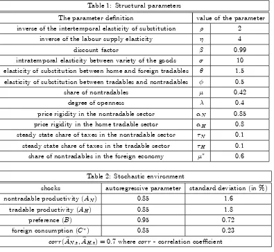
We summarize all parameters described above in Table 1 (Structural parameters) and Table 2 (Stochastic environment) in Appendix B. Moreover Table 3 (Matching the moments) in Appendix B compares the model moments with the historical moments for the Czech Republic economy.
6.2
Unconstrained optimal monetary policy
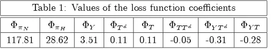
[image:23.612.120.392.503.553.2]Now, we characterize the optimal monetary policy under the chosen parameterization. First, we analyze what the main concern of the optimal monetary policy is by studying the coe¢cients of the loss function given by (38).30 In Table 1, we present these coe¢cients.
Table 1: Values of the loss function coe¢cients
N H Y Td T T Td Y Td Y T
117.81 28.62 3.51 0.11 0.11 -0.05 -0.31 -0.28
The highest penalty coe¢cient is assigned to ‡uctuations in nontradable sector in‡ation and home tradable in‡ation. Therefore, the optimal monetary policy mainly stabilizes domestic in‡ation. This …nding is in line with the literature on core in‡ation targeting (Aoki (2001)). Apart from that, the
2 9Empirical evidence shows that productivity shocks are highly persistent and positively correlated (see Backus et al
(1992)).
3 0Following Benigno and Woodford (2005), we check whether the second-order conditions of the policy problem are
optimal monetary policy faces a trade o¤ between stabilizing the output gap and the sector in‡ations which is re‡ected in the positive values of the penalty coe¢cients assigned to ‡uctuations in domestic and international terms of trade.
Next, we check whether the optimal monetary policy satis…es the Maastricht convergence criteria. Since the means of all variables under the optimal monetary policy are zero, we can reduce constraints (51)–(58) to the following set of inequalities:
d
var(bt) (K 1)B2 (65)
d
var(Rbt) (K 1)CR2 (66) d
var(Stb) (K 1)DS2; (67) wherevard(xt) =Et0
1
X
t=t0 tx2
t andxt=bt;Rt;b St:b Notice that these constraints set the upper bounds
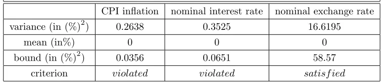
[image:24.612.117.496.379.461.2]on the variances of the Maastricht variables. In Table 2, we present variances of these variables under optimal monetary policy and the respective upper bounds that represent the right-hand side of equations (65)–(67). We write that a criterion is violated (satis…ed) when the variance of the respective Maastricht variable is higher (smaller) than the upper bound.
Table 2: Moments of the Maastricht variables under optimal monetary policy
CPI in‡ation nominal interest rate nominal exchange rate
variance (in (%)2) 0.2638 0.3525 16.6195
mean (in%) 0 0 0
bound (in (%)2) 0.0356 0.0651 58.57
criterion violated violated satisf ied
The optimal monetary policy violates two of the Maastricht convergence criteria, the CPI in‡ation criterion and the nominal interest rate criterion. The nominal exchange rate criterion is satis…ed.31 Therefore, the loss function of optimal monetary policy for the EMU accession countries must be augmented by additional terms.
6.3
Constrained optimal policy
Now, we construct the optimal monetary policy that satis…es all Maastricht criteria. First, we augment the loss function of the optimal monetary policy with additional terms re‡ecting ‡uctuations of CPI in‡ation and the nominal interest rate and solve the new policy problem.32 Second, we check whether such a policy also satis…es the nominal exchange rate criterion.
3 1Note that currently, the Czech Republic economy satis…es the Maastricht criteria regarding CPI in‡ation, the
nominal interest rate and the nominal exchange rate. See Figures 3 (the CPI in‡ation criterion), 5 (the nominal interest rate criterion) and 6 (the nominal exchange criterion) in Appendix A.
The loss function of the optimal policy that satis…es two additional constraints on CPI in‡ation and the nominal interest rate is given below:
e
Lt=Lt+
1 2 (
T
bt)2+
1 2 R(R
T Rb
t)2; (68)
where >0; R>0and T <0; RT <0:Values of the penalty coe¢cients ( ; R) and targets
( T; RT) can be obtained from the solution to the minimization problem of the original loss function
constrained by structural equations (39)–(42) and also the additional constraints on the CPI in‡ation rate (51)–(52) and the nominal interest rate (53)–(54).33 These values are presented in Table 3:
Table 3: Values of the additional parameters in the augmented loss function
R T (in %) RT (in %)
42.65 23.87 -0.1779 -0.1877
Notice that values of the penalty coe¢cients on the CPI in‡ation rate and nominal interest rate ‡uctuations are of the same magnitude as the penalty coe¢cients on the domestic in‡ation rates. The negative target value for the CPI in‡ation rate means that now, monetary policy targets the CPI in‡ation rate and the nominal interest rate that in annual terms are 0.7% smaller than their foreign counterparts.
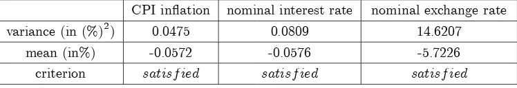
[image:25.612.122.496.486.550.2]Finally, we check whether this policy also satis…es the nominal exchange rate criterion. In Table 4, we present the …rst and second discounted moments of all Maastricht variables and evaluate whether each of the criteria is satis…ed. A criterion is satis…ed when the respective set of inequalities that describes this criterion holds. In particular, the CPI in‡ation criterion is described by the set of in-equalities (51)–(52), the nominal interest criterion is explained by (53)–(54) and the nominal exchange rate criterion by (55)–(58).
Table 4: Moments of the Maastricht variables under the constrained optimal policy
CPI in‡ation nominal interest rate nominal exchange rate
variance (in (%)2) 0.0475 0.0809 14.6207
mean (in%) -0.0572 -0.0576 -5.7226
criterion satisf ied satisf ied satisf ied
Importantly, the nominal exchange rate criterion is satis…ed. Not surprisingly, variances of the CPI in‡ation rate and the nominal interest rate are smaller than under the optimal policy. Notice that the variance of the nominal exchange rate is smaller than the one under the optimal monetary policy. This is due to the fact that the nominal exchange rate changes are, apart from the domestic sector in‡ation rates, one of the components of the CPI in‡ation rate (see (34)). So the policy that
3 3Special thanks to Michael Woodford for explaining the algorithm to …nd the parameters of the constrained policy
targets domestic in‡ation rates and the CPI aggregate in‡ation rate at the same time also decreases the nominal exchange rate variability. Let us remark that the negative targets for the nominal interest rate and the CPI aggregate in‡ation lead to negative means of all Maastricht variables. Therefore, a central bank choosing such a policy commits itself to a policy resulting in the average CPI in‡ation rate and the nominal interest rate being 0.2% smaller in annual terms than their foreign counterparts. Additionally, this policy is characterized by an average nominal exchange rate appreciation of nearly 6%.
Summing up, the optimal monetary policy constrained by additional criteria on the CPI in‡ation and the nominal interest rate is the policy satisfying all Maastricht convergence criteria.
6.4
Comparison of the constrained and unconstrained optimal policy
Now, we focus on the comparison of the optimal monetary policy and the optimal policy constrained by the convergence criteria. First, we calculate the welfare losses associated with each policy and second, we analyze di¤erences between the policies in their stabilization pattern when responding to the shocks.
In Table 5, we present the expected discounted welfare losses for both policies:
Table 5: Welfare losses for the unconstrained and constrained optimal policy
UOP COP
loss (in (%)2) 7.1533 9.2956
where UOP is the unconstrained optimal policy and COP is the constrained optimal monetary policy.
The obligation to comply with the Maastricht convergence criteria induces additional welfare costs equal to 30% of the optimal monetary policy loss. These welfare costs are mainly explained by the deterministic component of the constrained policy. Although the constrained optimal policy reduces variances of the Maastricht variables, it must also induce negative targets for the CPI in‡ation rate and the nominal interest rate to satisfy the criteria. These negative targets result in the negative means of all variables.
a de‡ationary bias feature of the constrained policy is preserved.34 These di¤erent values of targets and penalty coe¢cients will alter the welfare loss associated with the constrained optimal monetary policy. Importantly, the more volatile is the foreign economy (due to suboptimal policy or a volatile stochastic environment of the foreign economy) the smaller is the welfare loss associated with the constrained optimal policy.
[image:27.612.122.526.284.368.2]Now, we investigate how the two policies, constrained optimal monetary policy and unconstrained optimal monetary policy, di¤er when responding to the shocks. First, we analyze which shocks are most important in creating ‡uctuations of the Maastricht variables. In the table below, we present variance decomposition results for CPI aggregate in‡ation, the nominal interest rate and the nominal exchange rate. Since the variance decomposition structure does not change to any considerable extent with the chosen policy, we report results for the constrained policy.
Table 6: Variance decomposition of the Maastricht variables under the constrained policy
shocks:
variables: AN AH B C
CPI in‡ation 80% 2% 11% 7%
nominal interest rate 86% 7% 4% 3%
nominal exchange rate 75% 3% 20% 2%
Around 80% of the total variability of CPI aggregate in‡ation, the nominal interest rate and the nominal exchange rate are explained by domestic nontradable productivity shocks. This result is consistent with the literature on the sources of in‡ation di¤erentials in the euro area (Altisssimo et al (2004)). Notice that although parameters describing productivity shocks are similar in our setup, each of the productivity shocks has a di¤erent impact on the real exchange rate and therefore, on the Maastricht variables. This can easily be understood by analyzing the following equation, which relates the real exchange rate to domestic and international terms of trade (see (28), (30)):
d
RSt=b Tdtd bTctd+ (1 a)Tbt: (69)
Both domestic productivity shocks result in real exchange rate depreciation. However, the magni-tude of the real exchange rate depreciation di¤ers between the two shocks. Nontradable productivity shocks lead to a decline in the domestic terms of trade and a rise in the international terms of trade. Both changes have a depreciation e¤ect on the real exchange rate. On the other hand, domestic tradable productivity shocks result in a rise of both types of terms of trade. From equation (69) we see that increases in both types of terms of trade cancel out and lead to a small change in the real exchange rate. As a result, domestic nontradable productivity shocks lead to a stronger real exchange rate depreciation and therefore, larger changes in the nominal interest rate and the CPI in‡ation rate.
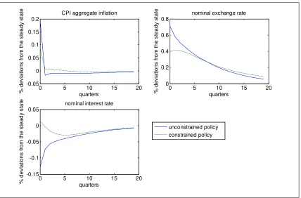
Having all this in mind, we decide to study the stabilization pattern of both policies in response to domestic nontradable productivity shocks.
0 5 10 15 20
-0.05 0 0.05 0.1 0.15 0.2
CPI aggregate inflation
quarters % d e v ia tio n s fro m th e s te a d y s ta te
0 5 10 15 20
0 0.2 0.4 0.6 0.8
nominal exchange rate
quarters % d e v ia tio n s fro m th e s te a d y s ta te
0 5 10 15 20
-0.15 -0.1 -0.05 0 0.05
nominal interest rate
[image:28.612.121.549.144.426.2]quarters % d e v ia tio n s fro m th e s te a d y s ta te unconstrained policy constrained policy
Figure 1: Impulse responses of the Maastricht variables to a positive domestic nontradable productivity shock
Under the unconstrained optimal policy, a positive domestic nontradable productivity shock leads to a fall in the nominal interest rate. This decrease of the nominal interest partially stabilizes de‡a-tionary pressures in the domestic nontraded sector and supports an increase in domestic aggregate output and consumption (not shown here). Since the foreign nominal interest rate remains constant, the uncovered interest rate parity induces a nominal exchange rate depreciation followed by an ex-pected appreciation. The initial nominal exchange rate depreciation results in a strong initial increase of CPI in‡ation, which declines in subsequent periods, reverting to its mean.