http://dx.doi.org/10.4236/ajcm.2015.54039
A New One-Twelfth Step Continuous Block
Method for the Solution of Modeled
Problems of Ordinary Differential Equations
Emmanuel Adegbemiro Areo, Micheal Temitope Omojola
Department of Mathematical Sciences, Federal University of Technology, Akure, Nigeria
Received 22 October 2015; accepted 13 December 2015; published 16 December 2015
Copyright © 2015 by authors and Scientific Research Publishing Inc.
This work is licensed under the Creative Commons Attribution International License (CC BY). http://creativecommons.org/licenses/by/4.0/
Abstract
In this paper, we developed a new continuous block method by the method of interpolation and collocation to derive new scheme. We adopted the use of power series as a basis function for ap-proximate solution. We evaluated at off grid points to get a continuous hybrid multistep method. The continuous hybrid multistep method is solved for the independent solution to yield a conti-nuous block method which is evaluated at selected points to yield a discrete block method. The basic properties of the block method were investigated and found to be consistent, zero stable and convergent. The results were found to compete favorably with the existing methods in terms of accuracy and error bound. In particular, the scheme was found to have a large region of absolute stability. The new method was tested on real life problem namely: Dynamic model.
Keywords
Power Series Approximate Solutions, Consistent, Zero Stability, Continuous Block Method, Dynamic Model
1. Introduction
In this paper, we considered the method of approximate solution of the general second order initial value problem of the form
(
, ,)
,( )
0,( )
y′′= f x y y′ y a =y y a′ =β (1)
Equation (1) is of interest to researchers because of its wide application in engineering, control theory and other real life problem, hence the study of the methods of its solution. Hence, authors proposed methods with different basis functions and among them are [1]-[9] to mention a few.
Block method was later proposed. This block method has the properties of Runge-kutta method for being self-starting and does not require development of separate predictors or starting values. Among these authors are [10]-[12]. Block method was found to be cost effective and gave better approximation.
In this paper, we propose a new one-twelfth step continuous hybrid block method for the numerical inte- gration of second order initial value problems with constant step-size which is then implemented in block mode.
The paper is organized as followed: Section 2 considers the mathematical formulation of the method. Section 3 considers the analysis of the basic properties of the method. Section 4 considers the Region of absolute stability of our method. Section 5 considers the application of the derived method to solve some second order Ordinary Differential Equations and conclusion.
2. Mathematical Formulation of the Method
We consider the simple power series as a basis function for approximation:
( )
1( )
0
,
r s j j j
Y x aφ x
+ −
=
=
∑
(2)where
φ
j( )
x =xjAnd x∈
[ ]
a b, , aj’s are coefficients to be determined and is a polynomial of degree r+ −s 1. We construct a k-step collocation method (MCM) by imposing the following conditions on (2)( )
n j n j, 0,1, 2, , 1Y x+ =y+ j= r− (3)
( )
n j n j, 0,1, 2, , 1Y′′ x+ = f + j= s− (4)
Substituting (1) into (4) gives
(
)
(
)
2, , 1 j
j
f x y y′ =
∑
j j− a x − (5)We shall consider a step-length of 1
12
k= with a constant step-size 1
48 h=
Interpolating (3) at 1
48 ,
n n
x x x
+
= and collocating (4) at 1 1 1 1
48 24 16 12
, , , ,
n
n n n n
x x x x x x
+ + + +
= gives a system of non-
linear equation of the form
AX =B (6)
where
[
]
T T
0 1 2 3 4 5 6 1 1 1 1 1
48 48 24 16 12
, , , , , , , n, , n, , , ,
n n n n n
A a a a a a a a B y y f f f f f
+ + + + +
= =
and
2 3 4 5 6
2 3 4 5 6
1 1 1 1 1 1
48 48 48 48 48 48
2 3 4
2 3 4 5
1 1 1 1
48 48 48 48
2 3 4
1 1 1 1
24 24 24 24
2 3 4
1 1 1 1
16 16 16 16
1 1
0 0 2 6 12 20 30
0 0 2 6 12 20 30
0 0 2 6 12 20 30
0 0 2 6 12 20 30
0 0 2 6
n n n n n n n n n n n n
n n n n
n n n n
n n n n
n n n n
x x x x x x
x x x x x x
x x x x
x x x x
X
x x x x
x x x x
x
+ + + + + +
+ + + +
+ + + +
+ + + +
=
2 3 4
1 1 1 1
12 12 12 12
12 20 30
n+ xn+ xn+ xn+
Solving (6) for the aj’s and substituting back into (3) and after much algebraic simplification, we obtained
0
2 2 2 2 2
1 1 1 1 1 1
48 24 16 12 48
2 2
2 2 2 2 2
3 1 1 1 1
48 24 16 12
2 2 2 2
4 1 1 1
12 16 2
1 47 29 7 367
48 48
128 11520 17280 23040 69120
1 2
32 50
32 24 2
3 3
280 88 448 912
n
n n
n n n n n
n
n n n n
n
n n n
a y
a h f h f h f h f h f y y
a h f
a h f h f h f h f h
a h f h f h f h f
+ + + + + + + + + + + + = = − + − + − + − = = − + − −
= + − + 2
1
4 48
2 2 2 2 2
5 1 1 1 1
48 24 16 12
2 2 2 2 2
6 1 1 1 1
48 24 16 12
832
41472 55296 32256 6912
2304
5 5 5 5
147456 221184 147456 36864 36864
5 5 5 5 5
n
n
n n n n
n
n n n n
h f
a h f h f h f h f h f
a h f h f h f h f h f
+ + + + + + + + + − = − + − − = − + − + + (7) where d 1 , d n
x x q
q
h x h
−
= = (8)
Evaluating (2) at 1 , 1 and 1
24 16 12
q= gives the main method below,
2 2 2 2 2
1 1 1 1 1/24 1
24 48 12 16 48
1 1 7 19 17
2
552960 138240 276480 552960 46080
n n n
n n n n n
y y y h f h f h f + h f h f
+ = − + + − + + + + + + + (9)
2 2 2 2 2
1 1 1 1 1 1
16 48 12 16 24 48
1 1 37 37 1
2 3
184320 17280 92160 552960 1280
n n
n n n n n n
y y y h f h f h f h f h f
+ = − + + − + + + + + + + + (10)
2 2 2 2 2
1 1 1 1 1 1
12 48 12 16 24 48
7 11 37 1 83
3 4
276480 23040 46080 10240 69120
n n
n n n n n n
y y y h f h f h f h f h f
+ = − + + + + + + + + + + + (11)
The Predictors are expressed as follows:
2 2 2 2 2
1 1 1 1 1
48 24 16 12 48
1 47 29 7 367
48 48
128 11520 17280 23040 69120
n n n
n n n n n
hy h f h f h f h f h f y y
+ + + + +
′ = − + − + − + − (12)
2 2 2 2 2
1 1 1 1 1 1
48 12 24 16 48 48
17 1 41 1 47
48 48
69120 512 n 11520 720 4320 n
n n n n n n
hy h f h f h f h f h f y y
+ + + + + +
′ = − + − + + + − (13)
2 2 2 2 2
1 1 1 1 1 1
24 12 24 16 48 48
1 97 37 13 361
48 48
13824 69120 n 3840 17280 17280 n
n n n n n n
hy h f h f h f h f h f y y
+ + + + + +
′ = + + − + + − (14)
2 2 2 2 2
1 1 1 1 1 1
16 12 24 16 48 48
11 119 263 1 3
48 48
23040 69120 n 11520 108 160 n
n n n n n n
hy h f h f h f h f h f y y
+ + + + + +
′ = − + + + + + − (15)
2 2 2 2 2
1 1 1 1 1 1
12 12 24 16 48 48
469 3 35 161 377
48 48
69120 2560 n 2304 5760 17280 n
n n n n n n
hy h f h f h f h f h f y y
+ + + + + +
′ = + + + + + − (16)
1 1 48 12 1 1 24 24 1 1 16 48 1 12 2
1 0 0 0 0 0 0 1
0 1 0 0 0 0 0 1
0 0 1 0 0 0 0 1
0 0 0 1 0 0 0 1
1 47 29 7
6144 552960 829440 1105920
1 1 1 1
1440 6912 12960 69120
13 102 n n n n n n n y y y y y y y y h + − + − + − = − − − − + 1 48 1 24 1 16 1 12 1 12 1 2 24 1 48
3 1 1
40 20480 6144 40960
1 1 1
0
540 2160 1620
367
0 0 0
3317760 53
0 0 0
207360 49
0 0 0
122880 7
0 0 0
12960 n n n n n n n n f f f f f f h f f + + + + − − − − + 1 12 1 24 1 48 1
0 0 0
48 1
0 0 0
24 1
0 0 0
16 1
0 0 0
12 n n n n y y h y y − − − ′ ′ + ′ ′ (17)
Writing (17) explicitly gives
2 2 2 2 2
1 1 1 1 1
48 48 24 16 12
1 47 29 7 367 1
6144 552960 829440 1105920 3317760 48
n n n
n n n n n
y y h f h f h f h f h f hy
+ = + + − + + + − + + + ′ (18)
2 2 2 2 2
1 1 1/24 1 1
24 48 16 12
1 1 1 1 53 1
1440 6912 12960 69120 207360 24
n n n n
n n n n
y y h f h f+ h f h f h f hy
+ = + + − + + − + + + ′ (19)
2 2 2 2 2
1 1 1 1 1
16 48 24 16 12
13 3 1 1 49 1
10240 20480 6144 40960 122880 16
n n n
n n n n n
y y h f h f h f h f h f hy
+ = + + + + + + − + + + ′ (20)
2 2 2 2
1 1 1 1
12 48 24 16
1 1 1 7 1
540 2160 1620 12960 12
n n n
n n n n
y y h f h f h f h f hy
+ = + + + + + + + + ′ (21)
Substituting (18) into (13)-(16) gives the following Block-Predictor as follows
1 1 1 1 1
48 48 24 16 12
323 11 53 19 251
17280 1440 17280 34560 34560 n n
n n n n n
y hf hf hf hf hf y
+ + + + +
′ = − + − + + ′ (22)
1 1 1 1 1
24 48 12 16 12
31 1 1 1 29
1080 180 1080 4320 4320 n n
n n n n n
y hf hf hf hf hf y
+ + + + +
′ = + + − + + ′ (23)
1 1 1 1 1
16 48 12 16 12
17 3 7 1 9
640 160 640 1280 1280 n n
n n n n n
y hf hf hf hf hf y
+ + + + +
′ = + + − + + ′ (24)
1 1 1 1 1
12 48 24 16 12
4 1 4 7 7
135 90 135 1080 1080 n n
n n n n n
y hf hf hf hf hf y
+ + + + +
3. Basic Properties of One-Twelfth Step Method
3.1. Order and Error Constant of the Block
Let the linear operator defined on the method be y x h
( )
; , Where,( )
( ) ( )0( )
( ) ( )2( )
( )
0
; ,
k
i i i
m n i n i m i
jh
y x h A Y y h d f y b F Y
i
−
=
∆ = −
∑
− + (26)Expanding the form Ym and F Y
( )
m in Taylor series and comparing coefficients of h, we obtained( )
( )
( )
( )
1 1( )
2 2( )
0 1 1 2
; p p p p p p
p p p
y x h C y x C hy x′ C h y x C +h + y + x C + h + y + x
∆ = + + + + + +
Definition: The linear operator and the associated block method are said to be of order p if
0 1 p p 1 0, p 2 0
C =C ==C =C + = C + ≠ . Cp+2 is called the error constant. It implies that the local truncation error is given by Tn k Cp 2hp 2yp 2
( )
x O h( )
p 3 .+ + +
+ = + +
Expanding the block in Taylor series expansion gives
2 2 0 0 2 2 0 0 1
1 367 1 1 47 1 29 1 7 1
48
! 48 3317760 ! 6144 48 552960 24 829440 16 1105920 12
1
1 53
24
! 24 207360 !
j
j j j j
j j
n n n n
j j
j
j j
n n n n
j j
h
y y hy h y
j j
h
y y hy h y
j j + ∞ ∞ = = + ∞ ∞ = = − − ′− ′′− − − − − − − ′− ′′− −
∑
∑
∑
∑
2 2 0 01 1 1 1 1 1 1 1
1440 48 6912 24 12960 16 69120 12
1
1 49 13 1 3 1 1 1 1 1
16
! 16 122880 ! 10240 48 20480 24 6144 16 40960 12
j j j j
j
j j j j
j j
n n n n
j j
h
y y hy h y
j j + ∞ ∞ = = − + + − − ′− ′′− − − − −
∑
∑
2 2 0 0 11 7 1 1 1 1 1 1
12
! 12 12960 ! 540 48 2160 24 1620 16
j
j j j
j j
n n n n
j j
h
y y hy h y
j j + ∞ ∞ = = − − ′− ′′− − − −
∑
∑
(27)Comparing the coefficients of h, the order of the block is p = 5
With error constant
T 2
107 1 1 1
, , , .
5917648890101760 23115815976960 14611478740992 11557907988480 p
C + =
3.2. Consistency
In numerical analysis, it is necessary that the method satisfies the necessary and sufficient conditions. A numerical method is said to be consistent if the following conditions are satisfies
1) The order of the scheme must be greater than or equal to 1 i.e. p≥1. 2)
0 0.
k j j=α =
∑
3) ρ
( )
r =ρ′( )
r =0. 4) ρ′′( )
r =2!σ( )
r .where, ρ
( )
r and σ( )
r are the first and second characteristics polynomials of our method. According to [3], the first condition is a sufficient condition for the associated block method to be consistent. Our method is order5
p= . Hence it is consistent.
3.3. Zero Stability of the Method
The general form of block method is given as( )0 ( ) ( ) ( )
1 1
i mu i i
m m m m
A Y =A Y − +h B Y +B Y − (28)
( )0 ( )
1 0 0 0 0 0 0 1
0 1 0 0 0 0 0 1
0
0 0 1 0 0 0 0 1
0 0 0 1 0 0 0 1
i A A λ λ − = − = 4 3
0, 0, 0, 0,1
λ −λ = λ=
Since no root has modulus greater than one and λ =1 is simple, the block method is zero stable in the 0.
h→
4. Region of Absolute Stability of the Block Method
According to Areo and Adeniyi [12], we express this stability matrix
( )
(
)
1M z = +V zB M−zA − U (29)
together with the stability function
( )
,(
( )
)
p η z =det ηI−M z (30)
Hence, we express the block method (18) in form of
( )
2
1 1
i i
Y A U h f y
Y+ B V Y−
− − − = − − − − − − − − − − − − (31)
0 0 0 0 0
367 1 47 29 7
3317760 6144 552960 829440 1105920
53 1 1 1 1
207360 1440 6912 12960 69120
49 13 3 1 1
122880 10240 20480 6144 40960
7 1 1 1
0
12960 540 2160 1620
367 1 47 29 7
3317760 6144 552960 829440 1105
A B − − − − = − − − =
( )
1 1 48 48 1 1 1 4824 24 1
1 1 16 16 1 1 12 12 0 1 0 1 0 1 920 0 1
7 1 1 1 0 1
0 0 1
12960 540 2160 1620
0 1 n n n n n n n i n n n n n V U y f y f y y f
Y f y Y
y y f y f + + + + + − + + + + = = = = = 1 48 1 1 12 n i n y Y y + + + = (32)
produce the required absolute stability region of the methods, as shown by the figure below
The graph Figure 1 shows that our method is A-Stable and the plot covers a large region of the complex plane z∈Cn.
5. Implementation of the Method
In this section, we discuss the strategy for the implementation of the method. In addition, the performance of the method is tested on some modeled examples of second order initial value problems in Ordinary Differential Equations. Absolute error of the approximate solution are then compared with the existing methods. In particular, the comparison are made with those proposed by Awoyemi et al. and Ehigie et al.
Discussion of the results of the methods are also done here.
5.1. Numerical Experiments
The method is tested on some numerical problems to test the accuracy of the proposed methods and our results are compared with the results obtained using existing methods.
The following problems are taken as test problems:
5.2. Implementation of the Method
5.2.1. Dynamic Problem
A 10-kg mass is attached to a spring having a spring constant of 140 N/m. The mass is started in motion from the equilibrium position with an initial velocity of 1 m/sec in the upward direction and with an applied external force F t
( )
=5sint. Find the subsequent motion of the mass if the force due to air resistance is −90xN .It follows from Newton’s second law
( )
mx= − −kx ax+F t (33)
or
( )
F t
a k
x x x
m m m
+ + =
(34)
[image:7.595.124.503.474.707.2]If the system starts at t = 0 with an initial velocity v0 and from an initial position x0, we also have the initial conditions.
( )
0 0,( )
0 0x =x x =v (35)
Now if m=10,k=140,a=90 and F t
( )
=5sint. The equation of motion, (28) becomes1
9 14 sin
2 x+ x+ x= t
(36)
Applying the initial conditions x
( )
0 =0 and x( )
0 = −1 to (30), we use the maple function( )
( )
( )
1( ) ( )
( )
9 14 sin , 0 0, 0 1
2
dsolvex t + x t + x t = t x = x = −
(37)
We get the exact solution
( )
9 2 99 7 9( )
13( )
e e cos sin
50 500 500 500
t t
x t = − − + − − t + t (38)
Note that the exponential terms, which come from the homogeneous solution represent an associated free overdamped motion, quickly die out. These terms are the transient part of the solution. The terms coming from the particular solution however, do not die out at t→ ∞; they are the steady-state part of the solution.
5.2.2. Problem 2
( )
( )
0, 0 0, 0 1, 0.1
y′′−y′= y = y′ = − h= (39)
Exact solution: y x
( )
= −1 exp( )
x .5.2.3. Problem 3
( )
( )
100 0, 0 1, 0 10, 0.01
y′′− y= y = y′ = − h= (40)
Exact solution: y x
( )
=exp(
−10x)
.5.2.4. Problem 4
( )
( )
0, 0 1 0 , 0.1
y′′+ =y y = =y′ h= (41)
Exact solution: y x
( )
=cos( )
x +sin( )
x .5.2.5. Problem 5
( )
2( )
( )
10, 0 1, 0 , 0.003125
2
y′′−x y′ = y = y′ = h= (42)
Exact solution: 1 1 2 .
2 2
x In
x
+
+
−
5.2.6. Problem 6
( )
2( )
π 1 3
2 , , π6
2 6 4 2
y
y y y y
y
′
′′= − = ′ =
(43)
Exact solution: y x
( )
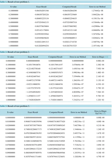
=sin2x.6. Conclusion
Table 1. Result of test problem 1.
X-value Exact Result Computed Result Error in our Method
0.10000000 −0.064362051546 −0.064362064290 1.274442e−08
0.20000000 −0.084307205226 −0.084307235669 3.044226e−08
0.30000000 −0.084052253134 −0.084052294635 4.150135e−08
0.40000000 −0.075293042133 −0.075293087518 4.538448e−08
0.50000000 −0.063570639604 −0.063570683902 4.429806e−08
0.60000000 −0.051421170694 −0.051421211160 4.046609e−08
0.70000000 −0.039930529564 −0.039930565039 3.547450e−08
0.80000000 −0.029498658628 −0.029498688913 3.028463e−08
0.90000000 −0.020212691313 −0.020212716720 2.540758e−08
1.00000000 −0.012026994254 −0.012027015325 2.107144e−08
Table 2. Result of test problem 2.
X-value Exact Result Computed Result Error in our Method Error in Ehigie [12]
0.00000000 0.000000000000 0.000000000000 0.0000000000 0.00E+00
0.10000000 −0.105170918076 −0.105170914197 3.878669e−09 3.38E−04
0.20000000 −0.221402758160 −0.221402741657 1.650316e−08 7.95E−04
0.30000000 −0.349858807576 −0.349858767673 3.990346e−08 1.40E−03
0.40000000 −0.491824697641 −0.491824622047 7.559449e−08 2.16E−03
0.50000000 −0.648721270700 −0.648721144076 1.266245e−07 3.13E−03
0.60000000 −0.822118800391 −0.822118604536 1.958546e−07 4.33E−03
0.70000000 −1.013752707470 −1.013752421828 2.856427e−07 5.79E−03
0.80000000 −1.225540928492 −1.225540528183 4.003098e−07 7.56E−03
0.90000000 −1.459603111157 −1.459602566974 5.441831e−07 9.70E−03
1.00000000 −1.718281828459 −1.718281106834 7.216251e−07 1.22E−02
Table 3. Result of test problem 3.
X-value Exact Result Computed Result Error in our Method Error in Ehigie Ey(7/4) [12]
0.00000000 0.0000000000000000 0.0000000000000000 0.000000+00 0.00E+00
0.01000000 0.9048374180359596 0.9048374180377620 1.802336e−12 4.08E−06
0.02000000 0.8187307530779818 0.8187307530850245 7.042700e−12 8.21E−06
0.03000000 0.7408182206817173 0.7408182206971640 1.544664e−11 1.24E−05
0.04000000 0.6703200460356393 0.6703200460624931 2.685374e−11 1.67E−05
0.05000000 0.6065306597126341 0.6065306597537941 4.115996e−11 2.12E−05
0.06000000 0.5488116360940276 0.5488116361518505 5.782286e−11 2.59E−05
0.07000000 0.4965853037914099 0.4965853038687461 7.733625e−11 3.09E−05
0.08000000 0.4493289641172210 0.4493289642167549 9.953394e−11 3.62E−05
0.09000000 0.4065696597405976 0.4065696598649566 1.243591e−10 4.18E−05
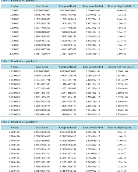
Table 4. Result of test problem 4.
X-value Exact Result Computed Result Error in our Method Error in Ehigie Ey(7/4) [12]
0.000000 0.000000000000 0.000000000000 0.000000e−00 0.00e−00 0.100000 1.094837581925 1.094837581922 3.099965e−12 4.25e−06 0.200000 1.178735908636 1.178735908611 2.533729e−11 8.46e−06 0.300000 1.250856695787 1.250856695772 1.497313e−11 1.26e−05 0.400000 1.310479336312 1.310479336286 2.533840e−11 1.66e−05 0.500000 1.357008100495 1.357008100457 3.748513e−11 2.04e−05 0.600000 1.389978088305 1.389978088254 5.069922e−11 2.40e−05 0.700000 1.409059874522 1.409059874458 6.442646e−11 2.74e−05 0.800000 1.414062800247 1.414062800169 7.796741e−11 3.06e−05 0.900000 1.404936877898 1.404936877807 9.066370e−11 3.34e−05 1.000000 1.381773290676 1.381773290574 1.018543e−10 3.59e−05
Table 5. Result of test problem 5.
X-value Exact Result Computed Result Error in our Method Error in Awoyemi et al. [6]
[image:10.595.89.537.374.648.2]0.00000000 0.000000000000 0.000000000000 0.000000e−00 0.0000e−00 0.10000000 1.050041729278 1.050041729278 3.086420e−14 2.6070e−13 0.20000000 1.100335347731 1.100335347731 2.420286e−13 1.9816e−09 0.30000000 1.151140435936 1.151140435936 8.442136e−13 6.5074e−09 0.40000000 1.202732554054 1.202732554052 2.102762e−12 1.5592e−08 0.50000000 1.255412811883 1.255412811879 4.368728e−12 3.1504e−08 0.60000000 1.309519604203 1.309519604195 8.227641e−12 5.6374e−08 0.70000000 1.365443754271 1.365443754257 1.439715e−11 9.6164e−08 0.80000000 1.423648930194 1.423648930170 2.408451e−11 1.5686e−08 0.90000000 1.484700278594 1.484700278555 3.921441e−11 2.4869e−08 1.00000000 1.549306144334 1.549306144271 6.294920e−11 3.8798e−08
Table 6. Result of test problem 6.
X-value Exact Result Computed Result Error in our Method Error in Ehigie Ey(7/4) [12]
0.52401544 0.250360930682 0.250360930682 1.515454e−14 000e−00 0.53401544 0.259074696912 0.259074696917 4.695411e−12 1.66e−09 0.54401544 0.267884830052 0.267884830070 1.825978e−11 4.70e−08 0.55401544 0.276787806164 0.276787806205 4.093692e−11 3.09e−07 0.56401544 0.285780064178 0.285780064251 7.270995e−11 5.45e−07 0.57401544 0.294858007310 0.294858007424 1.141097e−10 8.65e−07 0.58401544 0.304018004504 0.304018004668 1.646641e−10 1.28e−06 0.59401544 0.313256391883 0.313256392108 2.249845e−10 1.79e−06 0.61401544 0.331953526392 0.331953526767 3.750489e−10 2.42e−06 0.62401544 0.341404794918 0.341404795382 4.646992e−10 3.17e−06
also applied our method to the dynamic problem and the result is as displayed in Table 1.
References
Block Method as Predictors. Mathematical Theory and Modelling, 5, 10-26.
[2] James, A.A., Adesanya, A.O., Sunday, J. and Yakubu, D.G. (2013) Half-Step Continuous Block Method for the Solu-tions of Modeled Problems of Ordinary Differential EquaSolu-tions. American Journal of Computational Mathematics, 3, 261-269. http://dx.doi.org/10.4236/ajcm.2013.34036
[3] Adesanya, A.O., Odekunle, M.R. and James, A.A. (2012) Order Seven Continuous Hybrid Methods for the Solution of First Order Ordinary Differential Equations. Canadian Journal on Science and Engineering Mathematics, 3, 154-158.
[4] Badmus, A.M. and Mishehia, D.W. (2011) Some Uniform Order Block Methods for the Solution of First Ordinary Differential Equation. JNAMP, 19, 149-154.
[5] Fatokun, J., Onumanyi, P. and Sirisena, U.W. (2011) Solution of First Order System of Ordering Differential Equation by Finite Difference Methods with Arbitrary. JNAMP, 30-40.
[6] Awoyemi, D.O., Adebile, E.A., Adesanya, A.O. and Anake, T.A. (2011) Modified Block Method for the Direct Solu-tion of Second Ordinary Differential EquaSolu-tions. International Journal of Pure and Applied Mathematics, 181-188.
[7] Onumanyi, P., Sirisena, U.W. and Jator, S.A. (1999) Solving Difference Equation. International Journal of Computing Mathematics, 72, 15-27. http://dx.doi.org/10.1080/00207169908804831
[8] Areo, E.A., Ademiluyi, R.A. and Babatola, P.O. (2011) Three-Step Hybrid Linear Multistep Method for the Solution of First Order Initial Value Problems in Ordinary Differential Equations. JNAMP, 19, 261-266.
[9] Areo, E.A. and Adeniyi, R.B. (2013) A Self-Starting Linear Multistep Method for Direct Solution of Second Order Differential Equations. International Journal of Pure and Applied Mathematics, Bulgaria, 82, 345-364.
[10] Ibijola, E.A., Skwame, Y. and Kumleng, G. (2011) Formation of Hybrid of Higher Step-Size, through the Continuous Multistep Collocation. American Journal of Scientific and Industrial Research, 2, 161-173.
http://dx.doi.org/10.5251/ajsir.2011.2.2.161.173
[11] Bronson, R. and Costa, G. (2006) Differntial Equations. 3rd Edition, McGraw Hill, 115-121.