Application of Association Rule Mining to Help Determine the Process of Career Selection

Application of Association Rule Mining to Help

Determine the Process of Career Selection

Harini Peri

Information and Communication Technology Manipal Institute of Technology

Manipal, India

Preetham Kumar, PhD

HOD, Information and Communication Technology Manipal Institute of Technology

Manipal, India

ABSTRACT

The enormous data present at a university can be analyzed to generate useful information regarding the career paths chosen by students over the last few years. This information can not only be used by the students for analyzing the scope of their chosen career path but also by various authorities in analyzing

the present career trends and understanding the scope of improvement among the less chosen ones. Dynamic Itemset Counting algorithm is an Association Rule Mining Technique used to identify patterns from an enormous amount of data, such as the data present at a university’s repository. This model is an attempt towards uncovering hidden patterns. The generated results of the algorithm help in giving useful insights to decision makers in helping them make better and informed decisions.

Keywords

Preferred attribute, support, confidence, minimum support, dynamic itemset counting algorithm

1.

INTRODUCTION

In today’s world numerous carrier options are available for individuals. It can be very challenging for one to choose from these options. Apart from considering their individual interests there might be several other factors that should be taken into consideration before finalizing such a decision.

This can be achieved through efficient data analysis. Every year several students pass out from various universities across the country. They might come from diverse backgrounds and belong to various regions; they can possess different background education choosing different courses. By the end of their education they will be in numerous professions, working for different companies. This information collected by a university at the end of each batch is stored in its repository [13].

The current research aims at using this collected data in analyzing the career trends for specific background information selected. This is where data mining comes into picture. Data Mining is one of the most important phases of Knowledge Discovery in Databases (KDD) [6, 7], which aims at discovering interesting and useful patterns from large databases. Data Mining deals with uncovering hidden patterns and trends among the databases. Several techniques such as Association Rule Mining, Clustering, Classification, Outlier Analysis, etc., exist to mine data [2[[4][5][9]. Each of the above mentioned techniques when implemented through various algorithms on the database help in the KDD process.

An attempt was made to implement an efficient Association Rule Mining (ARM) algorithm. Dynamic Itemset Counting (DIC), is one of the existing efficient ARM algorithm, was initially used to analyze and convert the data present in a

repository into useful information. However, certain modifications were made to this approach to suit the current scenario in a much efficient way.

2.

ASSOCIATION RULE MINING

Association rule mining is a popular and well researched method for discovering interesting relations among variables in large databases. It uses different measures of interestingness to discover strong rules present in databases [3].

According to Agrawal et al [10], associations rule mining is defined as: Let I= (ι1, ι2, . . . , ιn ) be a set of binary attributes called items. Let T= (τ1, τ2… τn) be a set of transactions called the database. Each transaction in D has a unique transaction ID and contains a subset of the items in I. A rule is defined as an implication of the form X ⇒ Y where X,Y⊆I and X∩Y=φ. The sets of items (for short itemsets) and are called antecedent (left-hand-side or LHS) and consequent (right-hand-side or RHS) of the rule respectively [3]. The support supp(x) of an item (or itemset) x is the percentage of transactions from D in which that item or itemset occurs in the database. In other words, the support of an association rule X⇒Y is the percentage transactions T in a database where X ∪ Y ⊆ T. The confidence or strength c for an association rule X ⇒ Y is the ratio of the number of transactions that contain X ∪ Y to the number of transactions that contain X. An itemset X ⊆ J is frequent if X is present in the user defined number of transactions or X satisfies user defined minimum support. Frequent itemsets are important because they are the building blocks to obtain association rules with a given confidence and support [1].

3.

DYNAMIC ITEMSET COUNTING

ALGORITHM

complete database pass. Thus an itemset can be considered for counting at the next checkpoint instead of waiting until the end of the previous pass [11].

As the itemsets are counted they are marked in four different ways [13]:

• Solid box: contains confirmed frequent itemset - An itemset that exceeds the support threshold (minsupp) after a complete scan of the database

• Solid circle: contains confirmed infrequent itemset – Even after a complete scan of the database it is below minsupp

• Dashed box: contains suspected frequent itemset - an itemset that dint complete an entire scan of the database but exceeds the minsupp

• Dashed circle: contains suspected infrequent itemset - an itemset that dint complete an entire scan of the database and is below minsupp

The Dynamic Itemset Counting algorithm works as follows:

1. The empty itemset is marked with a solid box. All the 1-itemsets are marked with dashed circles. All other itemsets are unmarked.

2. Read M transactions. Experiments have been conducted with values of M ranging from 100 to 10,000. For each transaction, increment the respective counters for the itemsets marked with dashes.

3. If a dashed circle has a count that exceeds the support threshold, turn it into a dashed square. If any immediate superset of it has all of its subsets as solid or dashed squares, add a new counter for it and make it a dashed circle.

4. If a dashed itemset has been counted through all the transactions, make it solid and stop counting it.

5. If the transaction file is at the end of, rewind to the beginning.

6. If any dashed itemsets remain, go to step 2 [11].

This way Dynamic Itemset Counting [11] starts counting just the 1- itemsets and then quickly adds counters 2,3,4,...,k- itemsets. After just a few passes over the data (usually less than two for small values of M) it finishes counting all the itemsets. Ideally, it is better to have M as small as possible so that counting itemsets can start very early in step 3. However, it is better not to reduce M below 100 as steps 3 and 4 incur considerable overhead with very small values of M [11].

4.

PROPOSED METHODOLOGY

If the data is fairly homogeneous and for small values of M, Dynamic Itemset Counting takes very few passes. While if the data is non homogeneous or it is highly correlated it takes larger number of passes. It may not have been realized that the itemset is large until it has been counted in the most of the database. This effect can be reduced considerably with randomizing the order of the transactions [11].

4.1

Data Filtering

The data present at a university will be non-homogeneous data as it contains data belonging to numerous sources. However, before executing an algorithm on this data, non-homogeneous data was converted to non-homogeneous data. This was possible by comparing the values of the corresponding

attributes of the database with the values desired by the decision maker; accordingly they are marked true or false.

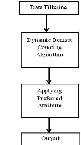
The steps involved in the proposed methodology are depicted in Figure 1.

Figure 1: Steps in the proposed methodology

Once this is achieved i.e., conversion of a non-homogeneous database to a homogeneous one, the number of different items will be equal to the total number of attributes. Although this involves one extra scan of the database, it filters out the unnecessary data even before the actual algorithm starts, thus optimizing the run time of the algorithm. A sample operation performed of this sort is depicted below:

Sample information selected by a decision maker:

Salary: 8-10 lakhs

Course: CS

Native State: -

College Location: Karnataka

Job Position: Software-Engineer

Background Education: MPC

College: MIT-Manipal

Gender: -

Company Location: -

Company: -

Table 1: Sample Database

ID 00001 00002 00003

Salary 10 6 3

Course CS IT BDS

Native State Andhra _Pradesh Kerala Goa

College

Location Karnataka Karnataka Delhi

Job Position Software _Engineer Software _Engineer Intern

Background

Education MPC MPC MBiPC

College MIT- _Manipal MIT-_Manipal AIIMS

Gender Male Female Female

Company

Location Andhra Pradesh Karnataka Delhi

Company Microsoft Tesco Apollo _Hospitals

4.2

Preferred Attribute

Once the data is mined from such a database, the usefulness of the data needs to be decided. The concept of using a preferred attribute will help ease this process.

Preferred attribute refers to that particular attribute which the decision maker chooses before executing the algorithm. It is a specific attribute selected by the decision maker among all the attributes that exist. For example, Course, College, Native State, etc. At the end of the execution of the algorithm, the preferred attribute is given preference and made sure it is matched in every single result set. Hence the rest of the result datasets although frequent are excluded out of the final result set as they are irrelevant to the end user.

Running the algorithm produces the results, which comprise of all the n-attribute sets; where ‘n’ represents the length of the dataset produced i.e., the number of attributes that match in the final result. If the final result has 8-attribute sets, then the closest matches to the profile are the profiles having 8 out of the 10 attributes in common.

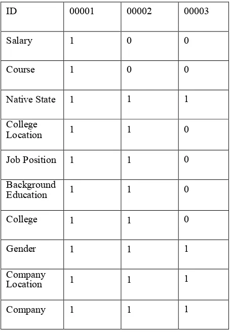
Table 2: Transformed Homogeneous Data

ID 00001 00002 00003

Salary 1 0 0

Course 1 0 0

Native State 1 1 1

College

Location 1 1 0

Job Position 1 1 0

Background

Education 1 1 0

College 1 1 0

Gender 1 1 1

Company

Location 1 1 1

Company 1 1 1

The data presented to the decision maker can be made more useful by filtering out only those results that contain the preferred attribute.

• If an individual is looking for a college only from a specific state, the name of the state has to be specified, along with the other information such as the course he desires to pursue, his background education etc., after setting the preferred attribute to ’College Location’ he can submit and view the results.

• Similarly if he desires to work only in a specific company, he can view all the colleges from which the company is hiring individuals.

• Check his job prospects after joining a particular college. This can be done by selecting the desired salary range like 10-16 lacks and set ‘College’ as preferred variable.

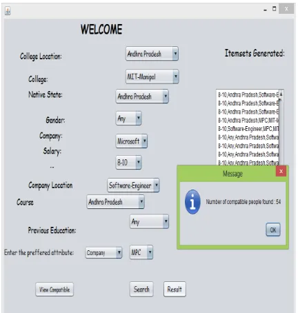
For example when an individual selects his information as follows:

Figure 2: Result after selecting the attributes

Figure 3: Viewing profile of identical individuals

By looking over the results tabulated in Table 3:

• The results provide profiles of students who match the specification provided by the decision maker. Thus providing a clear and complete overview.

• The experimental results give inputs to the decision makers on the trends in demand for the various courses, the educational background required for the desired course, the trends in selecting courses by students of a particular region etc. With the help of this information the student can prepare better for the course.

• Based on certain selective inputs that are common amongst many students, universities can analyze the results and can accordingly comprehend how appealing they are to the students.

• Demand for selected jobs in a particular region will indicate a high investment potential, attracting industries to invest and create employment.

The algorithm implemented above gave satisfactory results in terms of uncovering the hidden patterns.

Table 3: Sample Results

Sample Run Number

1 2 3 4

Native

State

- Andhra

Pradesh

Kerala -

Previous

Education

MPC - MEC MEC

Gender - - - -

Course CS Civil CA LLB

College MIT-

Manipal

- - -

College

Location

Karnatak a

Andhra

Pradesh

- -

Salary 10-16 lakhs

- - -

Job Position

Software

Engineer

- - Lawyer

Company - - - AZB

&

Partners

Company

Location

- - - Bangalor

e

Preferred

Attribute

Salary Native

State

Previous

Educatio n

Company

No of

Matches

64 301 214 40

Knowledge Mined: From Table 3, the following information can be inferred

1. The companies who visit a specified college and provide a remuneration which falls in the specified salary range

2. The number of students pursuing the specified course in a college belonging to the specified native state.

3. The list of people with similar profiles, the list of colleges that can be considered, job prospective after selecting that particular college, etc.

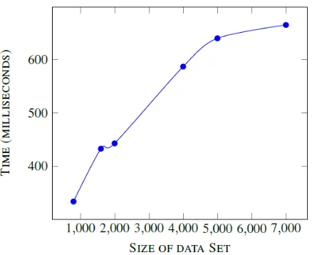
Figure 4: A graph showing the time required for execution of the algorithm for various dataset sizes.

From the graph shown in the Figure 4, it can be observed that the time required for the execution of the dataset increases as the size of the dataset increases and after crossing a certain threshold dataset size the execution time remains fairly constant. This stabilization of the execution time indicates the stability of the algorithm in terms of performance.

5.

CONCLUSION

While the original Dynamic Itemset Counting algorithm can be employed by a huge institution to compare the results on a larger scale the optimized version presented in this paper is perfectly suitable for its application in mining similar profiles as selected by the user.

While the original Dynamic Itemset Counting algorithm provides larger result sets which can be compared parallely, the improvised version in this paper provides only the information relevant to the user. This customization of information shown to the user is achieved by initially allowing the user to choose the attributes in accordance to the results he desires.

Thus, by utilizing the advantage of the situation and converting the non-homogeneous data into homogeneous data before the start of the algorithm the process is being optimized reducing the number of database scans.

6.

REFERENCES

[1] Anubha Sharma, Nirupma Tivari . 2012. “A Survey of Association Rule Mining Using Genetic Algorithm.” A Survey of Association Rule Mining Using Genetic Algorithm. Volume 1, Issue 2, pp 5-11.

[2] Bakar, Z.A. et al. 2006. “A Comparative Study for Outlier Detection Techniques in Data Mining.” IEEE Conference on Cybernetics and Intelligent Systems. Bangkok, 7-9 June 2006. IEEE, pp 1-6.

[3] Ila Chandrakar, and Mari Kirthima, A. 2013. ‘A Survey on Association Rule Mining Algorithms.” International Journal of Mathematics and Computer Research. Volume 1, Issue 10, pp 270-272.

[4] Sabarigirivason, K. et al. 2014. Association Rule Mining Based a Personalized Mobile Search Engine.’ International Journal of Advanced Research in Computer and Communication Engineering. Volume 3, Issue 1, pp 5272-5278.

[5] Mrs. Sonali Manoj Raut, Prof. Dhananjay Dakhane. 2012. “Comparative Study of Clustering and Association Method for Large Database in Time Domain.” International Journal of Advanced Research in Computer Science and Software Engineering. Volume 2, Issue 12.

[6] Numprasertchai, S. Poovaravan, Y. 2006. “Enhancing University Competitiveness through ICT Based Knowledge Management Systems.” IEEE Int. Conf. on Management of Innovation & Technology. Volume-1, pp 417–421,IEEE[Online].DOI: 10.1109/ ICMIT. 2006. 262196.

[7] Oded Maimon, Lior Rokach. 2005. “Introduction to Knowledge Discovery in Databases.” Data Mining and Knowledge Discovery Handbook, pp 1-17. Springer US [Online]. Available at: http://link.springer.com.

[8] Preeti Paranjape-Voditel, Dr.Umesh Deshpande. 2011. “A DIC-based Distributed Algorithm for Frequent Itemset Generation.” Journal of Software. Volume 6, Issue 2, pp 306-313.

[9] Qiankun Zhao, Nanyang Technological University, Singapore and Sourav, S. Bhowmick. 2003. “Technical Report on Association Rule Mining”: A Survey, No. 2003116. CAIS, Nanyang Technological University, Singapore.

[10] Rakesh Agrawal, Tomasz Imielinski, Arun, Swami, N. 1993. “Mining association rules between sets of items in large databases”. Proceedings of the 1993 ACM SIGMOD International Conference on Management , pp 207-216. Washington DC, USA.

[11] Sergey Brin et al. 1997. “Dynamic Itemset Counting and Implication Rules for Market Basket Data”. ACM SIGMOD International Conference on Management of Data,pp255-264[Online].DOI:10.1145/ 253262.253325.

[12] Sohil, Pandya. D and D. P. V. V. 2012. “Studying in impact of past performance in academics using data mining technique”. International Journal of Information and Computing Technology.