http://dx.doi.org/10.4236/jsip.2015.64024
Convolutional Noise Analysis via Large
Deviation Technique
Monika Pinchas
Department of Electrical and Electronic Engineering, Ariel University, Ariel, Israel
Received 8 September 2015; accepted 10 November 2015; published 13 November 2015
Copyright © 2015 by author and Scientific Research Publishing Inc.
This work is licensed under the Creative Commons Attribution International License (CC BY).
http://creativecommons.org/licenses/by/4.0/
Abstract
Due to non-ideal coefficients of the adaptive equalizer used in the system, a convolutional noise arises at the output of the deconvolutional process in addition to the source input. A higher con-volutional noise may make the recovering process of the source signal more difficult or in other cases even impossible. In this paper we deal with the fluctuations of the arithmetic average (sam-ple mean) of the real part of consecutive convolutional noises which deviate from the mean of or-der higher than the typical fluctuations. Typical fluctuations are those fluctuations that fluctuate near the mean, while the other fluctuations that deviate from the mean of order higher than the typical ones are considered as rare events. Via the large deviation theory, we obtain a closed-form approximated expression for the amount of deviation from the mean of those fluctuations consi-dered as rare events as a function of the system’s parameters (step-size parameter, equalizer’s tap length, SNR, input signal statistics, characteristics of the chosen equalizer and channel power), for a pre-given probability that these events may occur.
Keywords
Large Deviation Theory, Blind Equalization, Blind Deconvolution
1. Introduction
are near the mean value are well understood and investigated. By well understood we mean that it is well understood how to control the convolutional noise power (thus also the convolutional noise fluctuation near the mean) via the step-size parameter or equalizer’s tap length for instance. But up to now, those fluctuations of the convolutional noise that are larger than the typical ones (which are near the mean), which occur rarely, were not addressed.
The theory of large deviations is concerned with the exponential decay of probabilities of large fluctuations in random systems. These probabilities are important in many fields of study, including statistics, finance, and engineering, as they often yield valuable information about the large fluctuations of a random system around its most probable state or trajectory [11]. According to [12], the theory of large deviations deals with the pro- babilities of rare events (or fluctuations) that are exponentially small as a function of some parameters, e.g., the number of random components of a system, the time over which a stochastic system is observed, the amplitude of the noise perturbing a dynamical system or the temperature of a chemical reaction. The reader may refer also to [13]-[17] for further information on the theory of large deviations.
In this paper we address indirectly those fluctuations of the convolutional noise that are larger than the typical ones, which occur very rare. Namely, we consider the fluctuations of the arithmetic average (sample mean) of the real part of consecutive convolutional noises which deviate from the mean of order higher than the typical fluctuations. As already mentioned, typical fluctuations are those fluctuations that fluctuate near the mean, while the other fluctuations that deviate from the mean of order higher than the typical ones are considered as rare events. Via the large deviation theory, we obtain a closed-form approximated expression for the probability that these rare events may occur as a function of the step-size parameter, equalizers’s tap length, SNR, input signal statistics, characteristics of the chosen equalizer (based on a cost function where the error of the equalized output can be expressed as a polynomial function of order up to three), channel power and the amount of deviation from the mean. Based on this new expression we are able to evaluate approximately the amount of deviation from the mean of those fluctuations considered as rare events as a function of the system’s parameters (step-size parameter, equalizers’s tap length, SNR, input signal statistics, characteristics of the chosen equalizer and channel power), for a pre-given probability that these events may occur.
The paper is organized as follows: after having described the system under consideration in Section 2 we evaluate in Section 3 approximately the amount of deviation from the mean of those fluctuations considered as rare events as a function of the systems parameters (step-size parameter, equalizerss tap length, SNR, input signal statistics, characteristics of the chosen equalizer and channel power), for a pre-given probability that these events may occur. Section 4 is our conclusion.
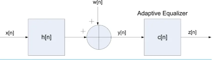
2. System Description
The system under consideration is illustrated in Figure 1, where we make the following assumptions:
1) The input sequence x n
[ ]
belongs to a two independent quadrature carrier case constellation input with variance σx2 where x nr[ ]
and x ni[ ]
are the real and imaginary parts of x n[ ]
respectively.2) The unknown channel h n
[ ]
is a possibly nonminimum phase linear time-invariant filter in which the transfer function has no “deep zeros”, namely, the zeros lie sufficiently far from the unit circle.3) The equalizer c n
[ ]
is a tap-delay line.4) The noise w n
[ ]
is an additive Gaussian white noise with zero mean and variance 2[ ] [ ]
w E w n w n
σ ∗
=
[image:2.595.133.501.606.710.2]where E
[ ]
⋅ is the expectation operator.The transmitted sequence x n
[ ]
is transmitted through the channel h n[ ]
and is corrupted with noise w n[ ]
. Therefore, the equalizer’s input sequence y n[ ]
may be written as:[ ] [ ] [ ]
[ ]
y n =x n ∗h n +w n (1) where “∗” denotes the convolution operation. The equalized output sequence is defined by:
[ ] [ ] [ ] [ ] [ ]
[ ]
z n =y n ∗c n =x n +p n +w n (2) where p n
[ ]
is the convolutional noise (convolutional error) due to non-ideal equalizer’s coefficients[ ] [ ]
[ ]
(
h n ∗c n ≠δ n)
and w n[ ]
=w n[ ] [ ]
∗c n . The update mechanism of the equalizer’s coefficients is given by[18]:
[
] [ ]
[ ]
[ ]
*[ ]
1 F z n
c n c n y n
z n
µ∂
+ = −
∂ (3)
where µ is the step-size parameter,
( )
⋅* stands for the conjugate operation and F z n[ ]
is a predefined cost function that characterizes the intersymbol interference, see [19]-[26]. Minimizing this F z n[ ]
with respect to the equalizer parameters will reduce the convolutional error. In the following we deal with thoseequalization methods where
[ ]
[ ]
F z n
z n
∂
∂ can be defined as a polynomial function P z n
[ ]
of order up tothree as is in the case of [19]. Thus, in this work we consider the following update mechanism of the equalizer’s coefficients:
[
] [ ]
[ ] [ ]
*1
c n+ =c n −µ P z n y n (4)
3. The Deviation from the Mean
In this section we obtain a closed-form approximated expression for the amount of deviation from the mean of those fluctuations considered as rare events as a function of the system’s parameters (step-size parameter, equalizers’s tap length, SNR, input signal statistics, characteristics of the chosen equalizer and channel power), for a pre-given probability that these events may occur.
Theorem 1. For the following assumptions:
1) The convolutional noise p n
[ ]
, is a zero mean, white Gaussian process with variance[ ] [ ]
2
2
p E p n p n mp
σ = ∗ =
, where mp = E p r2
[ ]
n . p nr[ ]
is the real part of p n[ ]
.2) The source signal x n
[ ]
is a complex input where the real part of x n[ ]
is independent with the imaginary part of x n[ ]
, with known variance 2x
σ and higher moments. The mean of the input sequence is zero. Namely, E x n
[ ]
= 0.3) The convolutional noise p n
[ ]
and the source signal are independent.4) F z n
[ ]
[ ]
z n
∂
∂ can be expressed as a polynomial function of the equalized output namely as P z n
[ ]
of order three.5) The gain between the source and equalized output signal is equal to one. 6) The convolutional noise p n
[ ]
is independent with w n[ ]
.The amount of deviation
( )
ps from the mean of those fluctuations considered as rare events as a function ofthe system’s parameters, given the probability that these events occur can be expressed by:
2 p s
rm p
M
≈ (5)
consecutive convolutional noises which deviate from the mean of order higher than the typical ones is expressed by:
[ ]
( )
1 1 exp M r s nP p n p r
M =
> ≈ −
∑
(6)and m is given according to p [27]:
1 1 1 2 1 1 1 2 1 1 1 2 1 1 1 2 2
1 1 1 1
1 1
1
2
1 1 1 1
1 2
1
for 0 and 0
min ,
or for 0
max , where 4 2 4 2 mp mp mp mp p mp mp mp mp p mp mp Sol Sol
m Sol Sol
Sol Sol
m Sol Sol
B B A C B
Sol
A
B B A C B
Sol A > > = ⋅ < = − + − = − − − = (7)
(
(
)
(
)
)
(
)
( )
( )
(
)
2 2 2 2 2
1 3 3 12 1 3 12 1 12 3 12
2 2 2
3 3 12 12
2 2
2 2 2 2 2 2 4 2
1 3 12 12 1 3 1 12 1 3
4 4 2 2 2
3 12 12 1 3 1
45 18 6 9 2 2 3
45 18 9
12 6 12 4 15
2 2 3
r r r
r
r r r r
r r
x x x
w
x x x x r
r r x x
A B a a a a a a a a a a
B a a a a
B B a a a a a a a a E x a
E x a a E x a a a a
σ σ σ
σ
σ σ σ σ
σ σ = + + + + − + + + + = + + + + + + + − + +
(
)
)
(
)
(
(
)
)
( )
(
)
(
)
2 2 4
2 3 3 12 12
2 2 2 2 2 2
3 3 12 1 3 12 1 12 12 3
2
2 2 2 4 2 4 2 2 4 6 2
1 1 12 1 3 12 12 1 3 3
2 2 6
3 3 12 12
45 18 9
90 36 12 18 4 2 6
2 2 2
15 6 3 45
r
r r r r
r r r r
r
w
x x x w
x x r x r x r r
w
B a a a a
B a a a a a a a a a a
C a a a E x a a E x a E x a a E x a
a a a a
σ
σ σ σ σ
σ σ σ σ
σ + + + + + + + + − − = + + + + + + + + +
(
)
(
( )
( )
)
[ ]
2 2 2 2 2 4
3 3 12 1 3 12 1 12
2
2 2 2 2 4 2 4
1 1 3 1 12 3 3 12 3 12
2
2 4 2 2 2
12 12
2
1 2
2
0
18 6 9 2
12 4 15 12 2
6
r r r r
r r r
r r
x x x w
x x r x r
r x w
k R
x
x k
k
a a a a a a a a
a a a a a a E x a a a a E x
a E x a N
B N h n
SNR
σ σ σ σ
σ σ σ
σ σ
µ σ
µ σ = −
= + + + + + + + + + + + + =
∑
+ (8)xr is the real part of x n
[ ]
, R is the channel length, N is the equalizer’s tap length,[ ]
2 2 2 1 0 r r xw k R
k k
SNR h n
σ
σ = −
=
=
∑
and a1, a12, a3 are properties of the chosen equalizer and found by:
[ ]
[ ]
(
1( )
r 3( )
r 3 12( )( )
r i 2)
F z n
Re a z a z a z z
z n
∂ =
+ +
∂
(9)
where Re
( )
⋅ is the real part of( )
⋅ and zr, zi are the real and imaginary parts of the equalized output[ ]
z n respectively.
Proof. Let us first define:
[ ]
1
1 M
M r
n
S p n
M =
Next, by using assumption 1 from this section, we may write:
[ ]
(
)
21 exp
2 2π
r
p p
d
f p n d
m m
= = −
(11)
The propability density function (pdf) for SM (10) is
(
)
exp 22π 2
M
p p
M Ms
f S s
m m
= = −
(12)
since a sum of Gaussian random variables is also exactly Gaussian-distributed. According to [11], a large deviation approximation is obtained from this exact result by neglecting the term M , which is subdominant with respect to the decaying exponential, thereby obtaining [11]
(
)
exp(
( )
)
;( )
22
M
p
s
f S s MJ s J s
m
= ≈ − = (13)
The Central Limit Theory (CLT) governs random fluctuations only near the mean-deviations from the mean
of the order of mp
M [14]. Fluctuations which are of the order of mp are, relative to typical fluctuations,
much bigger: they are large deviations from the mean [14]. They happen only rarely, and so large deviation theory is often described as the theory of rare events-events which take place away from the mean, out in the tails of the distribution; thus large deviation theory can also be described as a theory which studies the tails of distributions [14]. According to [11] [14], the probability that
(
M s)
exp(
( )
s)
P S > p −MJ p (14)
where according to [11], is used to stress that as M → ∞ the dominant part of P M1 nM=1p nr
[ ]
ps >
∑
isthe decaying exponential exp
(
−MJ p( )
s)
. Thus, based on (14), we may write:[ ]
( )
1 1
exp M
r s
n
P p n p r
M =
> −
∑
(15)where
( )
(
)
( )
exp −MJ ps ≈exp −r (16)
and
( )
sr J p
M
≈ (17)
Thus from (17) and (13) we have:
2 2
2
p s
s p
rm
p r
p
m ≈M ⇒ ≈ M (18)
Next we turn to find a closed-form approximated expression for mp. Based on [27], the expression for the
convolutional noise power mp for the noisy and non-biased input case
(
E x n[ ]
= 0)
is given by (7), (8) and(9). This completes our proof.
4. Conclusion
mean of those fluctuations considered as rare events as a function of the system’s parameters (step-size pa- rameter, equalizerss tap length, SNR, input signal statistics, characteristics of the chosen equalizer and channel power), for a pre-given probability that these events may occur.
Acknowledgements
We thank the Editor and the referee for their comments.
References
[1] Wang, J., Huang, H.N., Zhang, C.H. and Guan, J. (2009) A Study of the Blind Equalization in the Underwater Com-munication. WRI Global Congress on Intelligent Systems, 3, 122-125. http://dx.doi.org/10.1109/GCIS.2009.61
[2] Rao, W., Yuan, K.-M., Guo, Y.-C. and Yang, C. (2008) A Simple Constant Modulus Algorithm for Blind Equalization Suitable for 16-QAM Signal. 9th International Conference on Signal Processing, Beijing, 26-29 October 2008, 1963- 1966.
[3] Weber, R., Schulz, F. and Bohme, J.F. (2002) Blind Adaptive Equalization of Underwater Acoustic Channels Using Second-Order Statistics. OCEANS’02 MTS/IEEE, 4, 2444-2452. http://dx.doi.org/10.1109/OCEANS.2002.1192010
[4] Abrar, S. and Nandi, A.K. (2010) Adaptive Minimum Entropy Equalization Algorithm. IEEE Communications Letters, 14, 966-968. http://dx.doi.org/10.1109/LCOMM.2010.083110.101168
[5] Feng, C. and Chi, C. (1999) Performance of Cumulant Based Inverse Filters for Blind Deconvolution. IEEE Transac-tion on Signal Processing, 47, 1922-1935. http://dx.doi.org/10.1109/78.771041
[6] Malik, G. and Sappal, A.S. (2011) Adaptive Equalization Algorithms: An Overview. International Journal of Ad-vanced Computer Science and Applications, 2, 62-67. http://dx.doi.org/10.14569/IJACSA.2011.020311
[7] Pinchas, M. and Bobrovsky, B.Z. (2006) A Maximum Entropy Approach for Blind Deconvolution. Signal Processing (Eurasip), 86, 2913-2931. http://dx.doi.org/10.1016/j.sigpro.2005.12.009
[8] Pinchas, M. (2013) Symbol Error Rate as a Function of the Residual ISI Obtained by Blind Adaptive Equalizers. Per-vasive and Embedded Computing and Communication Systems (PECCS 2013), Barcelona, 19-21 February 2013. [9] Pinchas, M. (2010) A Closed Approximated Formed Expression for the Achievable Residual Intersymbol Interference
Obtained by Blind Equalizers. Signal Processing (Eurasip), 90, 1940-1962.
http://dx.doi.org/10.1016/j.sigpro.2009.12.014
[10] Pinchas, M. (2010) A New Closed Approximated Formed Expression for the Achievable Residual ISI Obtained by Adaptive Blind Equalizers for the Noisy Case. IEEE International Conference on Wireless Communications, Network-ing and Information Security WCNIS2010, Beijing, June 2010, 26-30. http://dx.doi.org/10.1109/wcins.2010.5541879
[11] Touchette, H. (2009) The Large Deviation Approach to Statistical Mechanics. http://arxiv.org/pdf/0804.0327v2.pdf
[12] Touchette, H. (2012) A Basic Introduction to Large Deviations: Theory, Applications, Simulations.
http://arxiv.org/pdf/1106.4146v3.pdf
[13] Duffy, K. and Metcalfe, A.P. (2004) The Large Deviations of Eestimating Rate-Functions. Applied Probability Trust.
http://www.hamilton.ie/ken_duffy/Downloads/tldoerf.pdf
[14] Lewis, J.T. and Russell, R. (1997) An Introduction to Large Deviations for Teletraffic Engineers.
http://www2.warwick.ac.uk/fac/sci/maths/people/staff/oleg_zaboronski/fm/large_deviations_review.pdf
[15] Varadhan, S.R.S. (2008) Large Deviations. The Annals of Probability, 36, 397-419.
http://dx.doi.org/10.1214/07-AOP348
[16] Shwartz, A. and Weiss, A. Large Deviations for Performance Analysis. http://webee.technion.ac.il/~adam/LD/intro.pdf [17] Dembo, A. and Zeitouni, O. (1998) Large Deviations Techniques and Applications. 2nd Edition, Springer, New York. [18] Nandi, A.K. (1999) Blind Estimation Using Higher-Order Statistics. Kluwer Academic Publishers, Boston, 66.
http://dx.doi.org/10.1007/978-1-4757-2985-6
[19] Godard, D.N. (1980) Self Recovering Equalization and Carrier Tracking in Two-Dimensional Data Communication System. IEEE Transactions on Communications, 28, 1867-1875. http://dx.doi.org/10.1109/TCOM.1980.1094608
[20] Shalvi, O. and Weinstein, E. (1990) New Criteria for Blind Deconvolution of Nonminimum Phase Systems (Channels). IEEE Transactions on Information Theory, 36, 312-321. http://dx.doi.org/10.1109/18.52478
[21] Pinchas, M. (2011) A MSE Optimized Polynomial Equalizer for 16QAM and 64QAM Constellation. Signal, Image and Video Processing, 5, 29-37. http://dx.doi.org/10.1007/s11760-009-0138-z
Transactions on Communications, 58, 1674-1685.
[23] Arenas-Garcia, J. and Figueiras-Vidal, A.R. (2006) Improved Blind Equalization via Adaptive Combination of Con-stant Modulus Algorithms. Proceedings of the IEEE Conference on Acoustics Speech and Signal Processing, Toulouse, 14-19 May 2006, 3. http://dx.doi.org/10.1109/ICASSP.2006.1660764
[24] Faruk, M.S. (2014) Modified CMA Based Blind Equalization and Carrier-Phase Recovery in PDM-QPSK Coherent Optical Receivers. Proceedings of the 16th International Conference on Computer and Information Technology, Khulna, 8-10 March 2014, 469-472. http://dx.doi.org/10.1109/ICCITechn.2014.6997333
[25] Jiang, Z.X., Zhang, M., Li, Z.C. and Lu, S.L. (2008) A Newly High-Speed MCMA Algorithm for QAM System. Pro-ceedings of the 4th International Conference on Wireless Communications, Networking and Mobile Computing, Dalian, 12-14 October 2008, 1-4.
[26] Liu, Y.Z. and Song, T. (2007) A New CMA Algorithm Based on Modified Conjugate Gradient. Proceedings of the In-ternational Conference on Wireless Communications, Networking and Mobile Computing, Shanghai, 21-25 September 2007, 1160-1162.
[27] Pinchas, M. (2015) Under What Condition Do We Get Improved Equalization Performance in the Residual ISI with Non-Biased Input Signals Compared with the Biased Version. Journal of Signal and Information Processing, 6, 79-91.