Financial Market Responses to Bank Indonesia’s Policy Announcements

Munich Personal RePEc Archive

Financial Market Responses to Bank

Indonesia’s Policy Announcements

Sahminan, Sahminan

Bank Indonesia

December 2007

Online at

https://mpra.ub.uni-muenchen.de/93401/

Financial Market Responses

to Bank Indonesia’s

Policy Announcements

Sahminan Sahminan

Bank Indonesia

Directorate of Economic Research and Monetary Policy

December 2007

Abstract

This paper examines the effect of the BI rate announcements on financial markets in Indonesia. The estimation results show that interbank interest rates with overnight, 1-week, and 1-month maturity are significantly lower a day before the announcement of lower BI-rate. On the other hand, the levels of exchange rate return, stock return, or

government bond’s yield are not significantly affected by BI-rate announcements. The announcements of lower or constant BI-rate significantly bring down volatility of interbank interest rate with overnight, 1-week, and 1-month maturity, as well as the

volatility of government bonds’ yield, exchange rate return and stock returns. The largest

effect of BI rate announcement is experienced by overnight interbank interest rate, both in terms of level as well as in terms of volatility.

JEL classification: E43, E44, E52, E58, C22

Keywords: Monetary Policy, Announcement, Bank Indonesia.

1. Introduction

In line with the growing implementation of inflation targeting framework since the 1990s, many central banks have moved toward more transparent policies. The need for a more transparent central bank has been accepted not only in academic but also in central banks. There is a broad consensus that transparency may help the effectiveness of policy (Woodford, 2003). Two key arguments stand out for the emphasis of the need for more transparent central bank. On normative side, as a public institution, independent central banks should meet high standard accountability through transparency. And from the conduct of monetary policy, it is viewed that the efficiency of monetary policy depends heavily on the credibility of central banks to implement inflation targeting framework and public perceptions of the consistency of central bank actions to achieve its announced targets (Heenan et al., 2006) The increase in the transparency itself is reflected in the increase in public communication by central banks.

Within inflation targeting frameworks, monetary policy communication is a key component, and inflation targeting central banks typically put much more effort into explaining the policy issues and decision, as well as more open about central bank activities. As pointed out by Heenan et al (2006), the main objectives of monetary policy communication is to convince economic agents—notably including financial market participants, price and wage setters, and fiscal authorities—that policy formulation and implementation is consistently oriented toward achieving inflation objective. Particularly for financial markets, the objectives of monetary policy announcement include ensuring that market participants are fully and simultaneously informed of any adjustments in policy instruments, ensuring that reporting and debate on monetary policy issues is well-informed, and promoting good understanding of monetary policy’s approach to policy formulation and risk assessment to maximize policy predictability.

makers to influence financial markets by moving asset prices in desired direction (market responsiveness). The hypothesis here is that if central bank is transparent then market should be able to anticipate policy decision rules well, that is, changes in asset prices on the announcement days should be small.

Recognizing the importance of transparency of an independent central bank, Bank Indonesia has moved toward a more transparent central bank since it obtained its independence from the government in 1999. The need for a more transparent central bank become even more crucial for Bank Indonesia since its implementation of inflation targeting framework started on July 2005. Since 1999 Bank Indonesia has taken various measures to be more open to the public regarding policies issues and decision as well as operations and research. In this respects, Bank Indonesia communicates with the public through various publications, Board’s speeches and testimonies, seminars, and discussions.

The purpose of this paper is to investigate the effect of Bank Indonesia’s policy announcements on financial markets in Indonesia. Specifically, we investigate how Bank

Indonesia’s monetary policy announcements affect inter-bank interest rates, exchange rate of the rupiah, stock return, and government bond’s yield in Indonesia. A better understanding on the effects of monetary policy announcement on financial markets will give a better understanding on the effectiveness of monetary policy undertaken.

The paper is organized as follows. Section 2 reviews monetary policy communication in Indonesia. Section 3 presents literature review. Section 4 discusses theoretical background of the announcement effects of monetary policy. Section 5 presents empirical models. Section 6 presents data and their descriptive statistics. Section 7 shows estimation results. Finally, this paper concludes with section 8.

2. Monetary Policy Communication in Indonesia

implementation of monetary policy. And in line with the increase in transparency and accountability, since July 2005 Bank Indonesia announces BI Rate following Board of Governor policy meeting every month.

As stipulated in Act No. 23, 1999 amended by Act No.3, 2004, Bank Indonesia’s

board of governor is required to hold monetary policy meeting at least once in a month. The policy meeting evaluates monetary policy undertaken and sets the direction of the monetary policy. The policy meeting is scheduled on first Tuesday or Thursday for every month following the day in which inflation rate is released by BPS (Statistics Indonesia). The BPS releases inflation rate on the first working day of every month. If for some reason the meeting cannot be held either on Tuesday or Thursday, the policy meeting is held on different pre-announced day. All policy meeting days are pre-announced publicly.

Table 1 shows the policy meeting days and BI decisions on BI rates. Since Bank Indonesia started using BI rate as a policy instrument until September 2007, there were 26 announcement days of BI rate, in which BI rate was raised five times, BI rate was cut 13 times and BI rate was kept unchanged eight times. Out of those 26 BI rate announcements, there is only incidence in which market expectation on BI rate was different from the announced BI rate, that is, on April 2007. Prior to the announcement on April 5, 2007, the median of market expectation on BI rate was 8.75 while the BI rate announced on April 5 was 9.00%2.

To avoid favoring some players in financial markets, the announcement of the policy meeting is released simultaneously, and since prompt information on BI rate is of great interest not only to domestic agents but also to foreigners, the press release on policy rate is published in both Bahasa Indonesia and English. As pointed out by Heenan et al (2002), international audiences of the policy announcement are also very important. International investors, portfolio managers, and foreign exchange strategists may not be well informed on the inflation targeting regime being into place that financial market may be more volatile than if such audiences were better informed. As background to its

2 _{The market expectation on BI rate is the expectation of a sample of large financial institutions provided by}

monthly policy statement, Bank Indonesia publishes a Monetary Policy Review in the months when a full inflation report has not been released by BPS.

Table 1: Bank Indonesia’s Press Release on BI Rate

Date Day Board of Governor Meeting’s (RDG) decision

July 5, 2005 Tuesday Sets BI rate for the first time, that is, at 8.5%

August 9, 2005 Tuesday Raises BI rate by 25 bps to 8.75%

September 6, 2005 Tuesday Raises BI rate by 125 bps to 10.00%

October 4, 2005 Tuesday Raises BI rate by 100 bps to 11.00%

November 1, 2005 Tuesday Raises BI rate by 125 bps to 12.25%

December 6, 2005 Tuesday Raises BI rate by 50 bps to 12.75%

January 9, 2006 Monday Keeps BI rate at 12.75%

February 7, 2006 Tuesday Keeps BI rate at 12.75%

March 7, 2006 Tuesday Keeps BI rate at 12.75%

April 5, 2006 Wednesday Keeps BI rate at 12.75%

May 9, 2006 Tuesday Cuts BI rate by 25 bps to 12.50%

June 6, 2006 Tuesday Keeps BI rate at 12.50%

July 6, 2006 Thursday Cuts BI rate by 25 bps to 12.25%

August 8, 2006 Tuesday Cuts BI rate by 50 bps to 11.75%

September 5, 2006 Tuesday Cuts BI rate by 50 bps to 11.25%

October 5, 2006 Thursday Cuts BI rate by 50 bps to 10.75%

November 7, 2006 Tuesday Cuts BI rate by 50 bps to 10.25%

December 7, 2006 Thursday Cuts BI rate by 50 bps to 9.75%

January 4, 2007 Thursday Curs BI rate by 25 bps to 9.50%

February 6, 2007 Tuesday Cuts BI rate by 25 bps to 9.25%

March 6, 2007 Tuesday Cuts BI rate by 25 bps to 9.00%

April 5, 2007 Thursday Keeps BI rate at 9.00%

May 8, 2007 Tuesday Cuts BI rate by 25 bps to 8.75%

June 7, 2007 Thursday Cuts BI rate by 25 bps to 8.50%

July 5, 2007 Thursday Cuts BI rate by 25 bps to 8.25%

August 7, 2007 Tuesday Keeps BI rate at 8.25%

September 6, 2007 Thursday Keeps BI rate at 8.25%

3. Literature Review

A large number of studies on the effects of macroeconomic announcements on financial markets can be found in the literature. And so far, most of the empirical studies on the announcement effects of monetary policy focus on the US and ECB monetary policy. Jones et al. (1998) examines the effects of announcements on the volatility of asset prices. They find that the volatility of asset prices on the announcement day does not persist, which is consistent with the immediate incorporation of information into prices. Unlike non-announcement shocks, shocks to volatility that occur on announcement days have no subsequent impact on daily volatility. When markets know that a large shock is forthcoming, return volatility in the market decreases.

Gurkayank et al. (2005) argue that viewing the effects of FOMC announcements on financial markets as driven by changes in federal fund rate target itself is inadequate. Instead, a second policy factor, which is the statements that the FOMC releases, accounted for more than three-fourth of the explaninable variation in the movements of five- and ten-year Treasury yield. When the decisions regarding the target for federal funds rate is not a surprise, changes in the wording of FOMC statements typically have been the major driver of financial market response.

Demirlap and Jorda (2004) investigate to what extent the policy of “the

announcement” affected a key ingredient in the monetary transmission mechanism, that is, the term structure of nominally risk-free, Treasury securities. They show that the movements of short-term interest rates tend be driven by public announcements by the Fed rather than liquidity changes as a result of open market operation

Bomfim (2000) examines how stock market in the US is affected by the Federal

Reserve’s scheduled policy announcements. He finds that stock market tends to be

relatively quite on days preceding regularly scheduled policy announcements, that is, the conditional volatility of stock return is abnormally low on those days. The element of surprise in actual interest rate decisions tends to boost stock market volatility significantly in the short run, and positive surprises tend to have a larger effect on volatility than negative surprises.

markets. They find that interest rates in US and euro area markets respond strongly to domestic monetary policy announcements. And interest rates in Germany and the euro area market react to Federal Reserve announcements in addition to European monetary policy announcements, while interest rates in US markets in general do not respond to European monetary policy announcements.

Rosa and Verga (2006) use tick-by-tick data to examine how ECB policy rate decision and the explanation of its monetary policy stance systematically hit financial markets the euro area. They find that unexpected component of ECB explanations significantly affect future prices and the impact is sizable. Their results suggest that financial markets seem to believe that the ECB does what it says it will do.

Among a few studies on the announcement effects of monetary policy other than that of the US or the ECB has been done, for example, by Guthrie and Right (2000). In their paper they develop theoretical as well as empirical models to analyze the effect of Reserve Bank of New Zealand (RBNZ) on interest rates in New Zealand. Their study show that the RBNZ has used communication systematically and effectively in controlling short-term interest rates.

Whereas a large literature exists on the response of monetary policy announcements on financial markets in industrialized countries, relatively little is known about the response of monetary policy announcement on financial markets in developing countries. This paper fills the gap in the literature by providing evidence on the effect of monetary policy announcements on financial markets in Indonesia.

4. Theoretical Background

monetary control if their objectives are less certain and have higher time preference, and therefore it takes longer for monetary policy to gain credible deflationary policy.

In another theoretical model, Guthrie and Wright (2000) analyze how central bank statements (open mouth operation) rather than open market operation leads to large changes in interest rates. Their model shows how the central bank can achieve inflation (and output) outcome without having to use open market operations to influence interest rates. Instead, as they show in their model, the central bank can achieve its objective by having a credible threat which ties down the level of interest rates. Without knowing the

central bank’s preferred rate, the private sector may deliver the wrong rate. This deviation

is costly from the central bank perspective.

By making an announcement (open mouth operation), the central bank can ensure the private sector delivers the correct rate. In choosing when to make such statements, the central bank trades off the flow costs of deviations away from its preferred level with the costs of making announcements. As central bank announcements release new information, each announcement should lead to a discrete jump in the level of interest rates in the desired direction. Moreover, using only publicly available information, announcements should be predictable—if the private sector could anticipate the released information, that information would already be incorporated in market rates.

The empirical implications of Guthrie and Wright’s (2000) theoretical model are as follows. First, an open mouth operation that released regularly represents a surprise to the private sector. If the market already knows that the central bank wants a change in monetary conditions, the market will already have delivered it. And second, interest rates of all maturities increase significantly following a tightening announcement, together with some appreciation of exchange rate. In another study specifically on financial markets, Ehrmann and Fratszcher (2007) argue that a credible monetary authority may be able to influence asset prices by communicating its views about its intended level and by signaling its intention to move policy if asset prices deviate from the target

Regarding the effects of monetary policy announcement on stock market, Bomfim (2003) argues that there are two possibilities in which the announcements affect stock market. First, there is a potential for pre-announcement effects which is commonly

of asset returns tend to be lower in days leading up to releases of major economic data

(“calming” effect) and then higher on the day of the announcement itself (“storm” effect).

And second, monetary policy decisions potentially affect market volatility through the nature of the decision itself. The announcement of the policy decision may reveal new information which is not previously incorporated into asset prices and volatility while participants process the newly received information.

5. Empirical Model

To measure the reactions of financial markets to Bank Indonesia’s policy announcement, we use Generalized Autoregressive Conditional Heteroscedasticity (GARCH) model. Similar model has also been used in many other studies on the effect of announcements on asset markets (see for example, Jones et al, 1998; Bomfim, 2003; and

Ehrmann and Fratzscher’s, 2007). The advantage of using exponential GARCH is that it corrects for the kurtosis, and skewness of the data. Considering that communication may influence both level and volatility of asset prices, we model both the influence of communication on asset price levels as well as the influence of communication on the volatility of asset prices.

Specifically, the base model is formulated as follows. Let R_t be the asset price returns then the relationship between asset price returns and announcement is given by:

t t

t t

t

t R D D D TUE THU

R ₀ _{1 1}_{1 1} ₂ _{3 1}₅ ₆  (1)

t t

t  h

 

THU TUE

D D

D h

h_t ₀ ₁_t2_1 _{2 t1}_{1 t1}_{2 t} _{3 t1} ₅ ₆

where _tis an independently identical distributed random variable with zero mean and unit variance,Dis a dummy for day in which BI policy rate is announced, TUEis dummy for Tuesday, and THUis dummy for Thursday.

0 1 6 0 5 0 1 4 1 3 2 1 1 1 1

0  

            

 t t t t t t t

t R D D D D D D

R        

t t

t

t D D TUE THU

D     

     

 

 



1 8 9 1 10 11

7 (4)

t t

t  h

  0 1 5 0 1 4 1 3 1 2 1 1 1 2 2 1 1

0  

              

 _{t t t t t t t}

t h D D D D D

h        

t t

t t

t D D D TUE THU

D      

            

 7 1 8 9 1 10 11

0 1 6

whereDis a dummy in which BI announces lower BI rate, D0 is a dummy in which BI announces keeps BI rate, and D is a dummy in which BI announces higher BI rate. The estimation uses Bollersev-Wooldridge robust quasi-maximum likelihood (QML) covariance/standard errors.

6. Data and Preliminary Analysis

Data on Bank Indonesia’s announcement on policy rates are obtained from Bank Indonesia’s website which is released every month following the policy meetings. Data on daily interest rates, exchange rates, and Jakarta Stock Market (JSX) Composite Index , and government-bond yield are obtained from CEIC database. Sample runs from July 1, 2005 to September 28, 2007. The starting date is chosen based on the fact that the use of BI rate as policy instrument started in July 2005. The advantage of using daily data is that it accounts for potential overshooting effects in the very short run (Ehrmann and Fratzscher, 2007). Moreover, since market participants are not necessarily clear about the exact time of the day in which monetary authority change the policy rate, using daily data instead of tick-by-tick data for the purpose of this study is reasonable.

Table 2: Descriptive Statistics of the Data

R_1N R_1W R_1M R_ER R_JSX SUN_1Y

Mean 7.76 8.92 10.82 -0.01 0.12 10.58

Median 7.48 8.93 10.89 0.00 0.13 10.64

Maximum 21.11 15.35 17.01 3.73 6.73 17.00

Minimum 3.50 3.59 3.69 -5.32 -6.65 2.31

Std. Dev. 3.02 2.53 2.11 0.56 1.33 2.06

Skewness 1.08 -0.01 -0.04 -0.72 -0.72 0.07

Kurtosis 4.43 1.69 1.83 22.58 8.32 2.28

Jarque-Bera 164.2 42.0 33.8 9391.0 739.6 12.99

Probability 0.00 0.00 0.00 0.00 0.00 0.00

Sum 4545.0 5226.4 6341.3 -6.6 72.8 6199.5

Sum Sq. Dev. 5322.3 3749.2 2608.3 179.9 1040.6 2482.5

Observations 586 586 586 585 585 586

Summary statistics of the data are presented in Table 2. The statistics of the interest rates show that while overnight rate has the lowest mean relative to 1-week and 1-month rates, the overnight rate has the highest standard deviation. This indicates that the overnight rate is more volatile relative to 1-week and 1-month rates. The information on the skewness and kurtosis of the data motivate the use of ARCH class of model in this paper. And the Jarque-Bera statistics show that for all series, the null hypothesis of a normal distribution is rejected at one percent significance level.

Table 3: Mean of the Data by Announcements

R_1N R_1W R_1M R_ER R_JSX SUN_1Y

All Days 7.76 8.92 10.82 -0.011 0.124 10.58

Non-Announcement (t) 7.75 8.91 10.81 -0.014 0.121 10.58

Announcement (t-1) 7.25 8.90 10.97 -0.027 0.239 10.53

Announcement (t) 7.88 9.16 11.04 0.050 0.190 10.59

Announcement (t+1) 7.51 9.32 10.97 -0.090 0.050 10.56

Announcement cut (t-1) 6.39 7.67 10.22 0.019 0.182 9.52

Announcement cut (t) 7.46 8.27 10.37 0.139 0.254 9.69

Announcement cut (t+1) 7.11 8.50 10.37 -0.057 0.235 9.70

Announcement keep (t-1) 7.96 9.42 10.98 0.122 -0.063 10.57

Announcement keep (t) 7.75 9.36 10.98 -0.098 -0.210 10.55

Announcement keep (t+1) 7.97 9.58 11.00 -0.106 -0.130 10.56

Announcement raise (t-1) 8.21 11.14 12.89 0.098 0.736 13.05

Announcement raise (t) 9.23 11.13 12.89 -0.415 0.931 12.99

Announcement raise (t+1) 7.71 11.00 12.45 -0.148 -0.093 12.77

Table 4: Standard Deviation of the Data by Announcements

R_1N R_1W R_1M R_ER R_JSX SUN_1Y

All Days 3.02 2.53 2.11 0.555 1.335 2.06

Non Announcement (t) 3.05 2.54 2.10 0.558 1.346 2.06

Announcement (t-1) 2.31 2.62 2.30 0.052 1.268 2.19

Announcement (t) 2.33 2.46 2.37 0.490 1.100 2.11

Announcement (t+1) 2.50 2.65 2.13 0.570 1.270 2.08

Announcement cut (t-1) 1.35 1.96 1.65 0.486 0.765 1.58

Announcement cut (t) 2.00 1.87 1.65 0.358 0.881 1.45

Announcement cut (t+1) 2.34 2.49 1.67 0.586 1.374 1.48

Announcement keep (t-1) 2.60 2.62 2.50 0.455 1.864 2.23

Announcement keep (t) 2.11 2.59 2.49 0.647 1.437 2.29

Announcement keep (t+1) 3.01 2.75 2.49 0.387 1.413 2.34

Announcement raise (t-1) 3.33 2.77 2.70 0.634 0.968 1.60

Announcement raise (t) 3.39 2.79 3.20 0.499 0.782 1.53

For exchange rate, the average of exchange rate return is higher when the announced BI rate is lower, and the average exchange rate return is lower when the

announced BI rate is higher or doesn’t change. The average stock return is also higher

when announced BI rate is lower or higher, but the average is lower when the announced BI rate doesn’t change. And the average of government-bond yield is lower when

announced BI rate is lower or doesn’t change, and higher when the announced BI rate is

higher. Standard deviations of exchange rate return and stock return are lower when announced BI rate is lower or higher, but the standard deviation is higher then the

announced BI rate doesn’t change. Meanwhile, standard deviation of government-bond yield is lower when BI rate is either higher or lower.

Figure 1: Mean and Standard Deviation of Interest Rates by Day of the Week (a) Overnight 7.30 7.40 7.50 7.60 7.70 7.80 7.90 8.00 8.10

Monday Tuesday Wednesday Thursday Friday 2.50 2.60 2.70 2.80 2.90 3.00 3.10 3.20 3.30 3.40 Mean (LHS) Std Dev (RHS)

(b) 1-Week 8.65 8.70 8.75 8.80 8.85 8.90 8.95 9.00 9.05

Monday Tuesday Wednesday Thursday Friday

2.49 2.50 2.51 2.52 2.53 2.54 2.55 2.56 2.57 2.58 2.59 Mean (LHS) Std Dev (RHS)

(c) 1-Month 10.65 10.70 10.75 10.80 10.85 10.90 10.95

Monday Tuesday Wednesday Thursday Friday

Figure 2: Mean and Standard Deviation of Exchange Rate Return, Stock Returns, Government Bond’s Yield by Day of the Week

(a) Exchange Rate Return

-0.10 -0.08 -0.06 -0.04 -0.02 0.00 0.02 0.04 0.06

Monday Tuesday Wednesday Thursday Friday

0.00 0.10 0.20 0.30 0.40 0.50 0.60 0.70 0.80

Mean (LHS) Std Dev (RHS)

(b) Stock Return

0.00 0.05 0.10 0.15 0.20 0.25

Monday Tuesday Wednesday Thursday Friday 0.00 0.20 0.40 0.60 0.80 1.00 1.20 1.40 1.60 1.80 Mean (LHS) Std Dev (RHS)

(c) G-Bond's Yield

10.44 10.48 10.52 10.56 10.60 10.64 10.68

7. Estimation Results

The most commonly used model of financial asset return volatility is the GARCH (1,1). The advantage of GARCH specification over ARCH specification is parsimony in identifying the conditional variance in GARCH (Wang, 2003). Moreover, GARCH models provide approximate descriptions of conditional volatility for a wide variety of volatility process (Jones, 1998). As discussed in section 5, two model specifications are estimated: (i) the model without taking into account direction of the change in BI rate; and (ii) the models separating the effects of the announcement based on the direction of the change in BI rate. The estimation results for those two model specifications are as follows.

7.1. Interest Rates

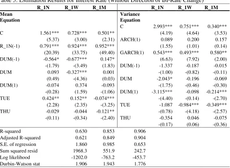
As shown in Table 5, interbank interest rate with 1-week maturity is significantly lower on the announcement day. A day before the announcement, interbank interest rates are significantly lower for overnight, and 1-week maturity, at least at 10 percent significance level. On the other hand, none of the interest rates is significantly lower for a day after the announcement. The effects of Tuesday or Thursday on interest rates are mixed, that is, on Tuesday interest rate is significantly higher for overnight and 1-week maturity, and it is significantly lower for 1-month maturity. On Thursday, only interest rate for 1-month that is significantly lower.

Table 5: Estimation Results for Interest Rate (without Direction of BI-Rate Change)

R_1N R_1W R_1M R_1N R_1W R_1M Mean

Equation

Variance Equation

C 2.993*** 0.751*** 0.340*** C 1.561*** 0.728*** 0.501** (4.19) (4.64) (3.53) (5.37) (3.00) (2.31) ARCH(1) 0.089 0.200 0.157 R_1N(-1) 0.791*** 0.924*** 0.952*** (1.55) (1.01) (0.14) (20.39) (33.75) (49.40) GARCH(1) 0.543*** 0.493*** 0.580** DUM(-1) -0.564* -0.677*** 0.147* (6.63) (7.92) (2.00) -(1.79) -(3.49) (1.83) DUM(-1) -1.337 -0.187 -0.015 DUM 0.093 -0.327*** 0.001 -(1.00) -(0.82) -(0.11) (0.49) -(4.36) (0.03) DUM -2.043* -0.196 -0.069 DUM(1) -0.074 0.374 -0.093 -(1.75) -(0.46) -(0.30) -(0.28) (1.59) -(1.06) DUM(1) -3.115*** -0.098 -0.214*** TUE 0.424** 0.152** -0.074*** -(4.40) -(0.14) -(2.70) (2.28) (2.35) -(3.25) TUE -1.087 -0.984*** -0.349*** THU -0.029 -0.044 -0.121** -(0.78) -(4.18) -(2.57) -(0.11) -(0.34) -(2.40) THU -0.354 0.046 -0.075 -(0.17) (0.06) -(0.36) R-squared 0.630 0.853 0.906

Adjusted R-squared 0.621 0.849 0.904 S.E. of regression 1.860 0.985 0.653 Sum squared resid 1968.3 551.9 242.7 Log likelihood -1202.0 -763.2 -453.7 Durbin-Watson stat 1.906 1.943 1.776

Notes: Numbers in the parentheses are z-statistics with Bollerslev-Wooldridge robust standard error. ***) significant at 1%; **) significant at 5%; *) significant at 10%.

In Table 6 we show the results of the estimation of the interest rate models in which the announcements are broken down based on the direction of the policy, that is, BI rate is cut, BI rate doesn’t change, and BI rate is raised. A day before the announcement of a lower BI rate the interbank interest rates for overnight, week, and 1-month maturity are significantly lower. On the announcement day, however, the announcement of unchanged BI-rate is only significantly for 1-week interbank rate, and the effect is negative.

Looking at the volatility of interest rates, on the announcement day the volatility of interest rate is significantly lower for 1-month maturity if BI rate is cut and for 1-week and 1-month maturity if BI rate doesn’t change. On the day before the announcement, the volatility of interest rates with 1-week and 1-month maturity is significantly lower when

rate is significantly lower for overnight and 1-month maturity if BI rate is cut; for overnight, 1-week, and 1-month maturity if BI rate doesn’t change; and for overnight maturity if BI rate is raised. Finally, day-of-the-week effect doesn’t have a significant effect on interest volatility.

Table 6: Estimation Results for Interest Rate (with Direction of BI-Rate Change)

R_1N R_1W R_1M R_1N R_1W R_1M

Mean Equation Variance Equation

C 1.599*** 0.684*** 0.548*** C 2.898 0.861*** 0.375*** (5.08) (3.46) (4.00) (1.51) (4.50) (10.04) R_1N(-1) 0.786*** 0.921*** 0.950*** ARCH(1) 0.078 0.141 0.156 (21.06) (42.04) (102.52) (1.15) (1.27) (0.25) DUM_NEG(-1) -1.148*** -0.640*** -0.181*** GARCH(1) 0.487 0.573*** 0.579*** -(2.84) -(2.99) -(4.00) (1.41) (8.88) (5.64) DUM_NEG -0.049 -0.152 0.020 DUM_NEG(-1) -2.251 -1.016*** -0.385*** -(0.15) -(0.67) (0.80) -(1.13) -(3.07) -(10.35) DUM_NEG(1) -0.002 0.408 -0.041 DUM_NEG -2.185 -0.756 -0.403*** -(0.01) (0.95) -(0.43) -(1.55) -(0.79) -(3.56) DUM_NOL(-1) 0.312 0.100 0.012 DUM_NEG(1) -3.778*** -0.196 -0.514*** (0.64) (1.36) (0.17) -(5.58) -(0.14) -(4.12) DUM_NOL -0.130 -0.185*** -0.012 DUM_NOL(-1) -1.485 -0.825*** -0.377*** -(0.59) -(2.55) -(0.14) -(0.90) -(4.44) -(10.06) DUM_NOL(1) -0.192 0.064 0.004 DUM_NOL -2.049 -0.638** -0.288* -(0.52) (0.80) (0.06) -(1.05) -(2.35) -(1.80) DUM_POS(-1) -0.830 -0.226 0.271 DUM_NOL(1) -2.789* -0.661*** -0.276*** -(1.09) -(0.47) (0.21) -(1.72) -(2.69) -(3.10) DUM_POS 0.904 0.019 0.412 DUM_POS(-1) 0.365 0.088 0.040 (1.16) (0.01) (0.20) (0.09) (0.01) (0.01) DUM_POS(1) 0.518 0.638 0.292 DUM_POS 0.329 0.126 0.061 (0.79) (0.95) (0.38) (0.16) (0.11) (0.11) TUE 0.458** 0.096 -0.055** DUM_POS(1) -5.539*** 0.105 0.036 (2.07) (1.46) -(2.11) -(7.09) (0.15) (0.08) THU 0.105 -0.046 -0.085** TUE -1.001 -0.346 -0.149 (0.36) -(0.35) -(2.53) -(0.85) -(1.10) -(1.01) THU -0.106 -0.062 -0.081 -(0.07) -(0.12) -(0.66) R-squared 0.632 0.856 0.909

Adjusted R-squared 0.615 0.849 0.905 S.E. of regression 1.874 0.984 0.651 Sum squared resid 1956.8 539.7 236.4 Log likelihood -1187.2 -825.3 -457.0 Durbin-Watson stat 1.902 1.939 1.778

7.2. Exchange Rate Return, Stock Return and Government Bond’s Yield

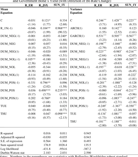
The model without breaking down the announcement does not show significant effect on the announcement on either exchange rate return or stock return both in level and in volatility (Table 7). However, when we breakdown the announcement based on the direction of the BI rate, in some cases the effect of the announcement is significant (Table 8). A day before the announcement in which the BI rate does not change, exchange rate return is significantly higher, and on the day of the announcement and a day before the announcement of higher BI rate, stock return is significantly higher. But the stock return is significantly lower a day after the announcement of higher BI rate. For

government bond’s yield, a day before the announcement of lower BI rate, the yield on

government bond is significantly lower, but on the day that BI rate is announced higher, the yield on government bond is significantly higher.

Table 7: Estimation Results for Exchange Rate Return, Stock Return

and Government Bond’s Yield (without Direction of BI Rate Change)

R_ER R_JSX SUN_1Y _{R_ER R_JSX} SUN_1Y

Mean Equation

Variance Equation

C -0.013 0.202*** _{0.195 C 0.033}* _{0.108 0.157}***

-(0.56) (3.63) (0.91) (1.74) (1.06) (7.42)

R_1N(-1) -0.013 0.126** _0.980***

ARCH(1) 0.293*** _0.297*** _1.610

-(0.19) (2.39) (59.18) (3.86) (3.60) (1.09)

DUM(-1) 0.011 -0.197 0.042 GARCH(1) 0.666*** _0.608*** _0.034

(0.16) -(1.03) (1.25) (10.58) (7.58) (0.50)

DUM 0.007 -0.022 0.097 DUM(-1) -0.024 0.270 -0.127***

(0.11) -(0.11) (1.47) -(0.85) (1.06) -(5.82)

DUM(1) 0.035 -0.113 0.056 DUM -0.063 -0.433 -0.087***

(0.43) -(0.48) (1.12) -(1.29) -(1.17) -(3.91)

TUE -0.039 -0.067 0.006 DUM(1) 0.047 0.484 -0.118***

-(0.94) -(0.54) (0.19) (0.70) (0.90) -(7.12)

THU -0.010 0.027 -0.019 TUE -0.017 0.369 -0.046***

-(0.22) (0.24) -(0.23) -(0.40) (1.55) -(3.55)

THU -0.044 0.060 0.025

-(1.12) (0.24) (0.47)

R-squared -0.002 0.000 0.944

Adjusted R-squared -0.027 -0.025 0.943

S.E. of regression 0.563 1.353 0.493

Sum squared resid 180.1 1040.1 138.2

Log likelihood -344.8 -920.5 -227.5

Table 8: Estimation Results for Exchange Rate, Stock Returns

and Government Bond’s Yield (with Direction of BI-Rate Change)

R_ER R_JSX SUN_1Y R_ER R_JSX SUN_1Y Mean

Equation

Variance Equation

C -0.031 0.121* 0.334 C 0.246*** _1.428*** _0.223***

-(1.14) (1.77) (2.68) (3.71) (4.95) (6.33) R_1N(-1) -0.046 0.104** 0.968*** ARCH(1) 0.160 0.142*** _0.123

-(0.87) (1.99) (90.32) (1.55) (2.52) (1.61) DUM_NEG(-1) -0.001 -0.053 -0.240* GARCH(1) 0.531*** _0.505*** _0.567***

-(0.01) -(0.23) -(1.88) (3.23) (4.14) (8.26) DUM_NEG 0.007 0.057 0.016 DUM_NEG(-1) -0.198*** _-1.040** _-0.083

(0.15) (0.27) (0.35) -(2.79) -(2.45) -(0.52) DUM_NEG(1) -0.046 -0.020 -0.089 DUM_NEG -0.223*** _-0.985* _-0.216***

-(1.19) -(0.06) -(1.51) -(2.64) -(1.94) -(2.07) DUM_NOL(-1) 0.105** -0.180 0.011 DUM_NEG(1) -0.194 -0.589 -0.385***

(2.36) -(0.43) (0.29) -(1.38) -(0.63) -(7.51) DUM_NOL -0.055 -0.344 -0.011 DUM_NOL(-1) -0.193*** _{-0.618 -0.228}***

-(0.38) -(0.91) -(0.28) -(4.87) -(1.03) -(6.45) DUM_NOL(1) -0.114 -0.162 -0.238 DUM_NOL -0.119 -0.105 -0.222*

-(0.93) -(0.49) -(1.68) -(1.54) -(0.28) -(1.81) DUM_POS(-1) -0.331 0.796** 0.096 DUM_NOL(1) -0.201** _-1.088** _-0.128

-(1.24) (2.02) (1.58) -(2.39) -(2.22) -(1.24) DUM_POS 0.036 0.498*** 0.235*** DUM_POS(-1) -0.080 -0.844* _-0.211***

(0.17) (3.73) (3.03) -(0.61) -(1.69) -(5.96) DUM_POS(1) 0.202 -0.760* 0.184 DUM_POS -0.096 -1.083*** _-0.247**

(0.85) -(1.68) (1.33) -(0.85) -(2.71) -(2.18) TUE 0.040 -0.048 0.025 DUM_POS(1) -0.249* _-1.367** _-0.350***

(0.75) -(0.40) (0.77) -(1.92) -(2.20) -(4.50) THU -0.008 0.047 -0.098*** TUE -0.134* _-1.081*** _-0.057

-(0.16) (0.37) -(2.13) -(1.73) -(3.00) -(0.48) THU -0.181*** _-1.188*** _-0.011

-(2.80) -(3.70) -(0.08)

R-squared 0.016 0.011 0.945 Adjusted R-squared -0.030 -0.035 0.943 S.E. of regression 0.564 1.360 0.493 Sum squared resid 176.9 1028.4 135.5 Log likelihood -431.8 -954.6 -387.2 Durbin-Watson stat 2.183 2.031 2.590

Notes: Numbers in the parentheses are z-statistics with Bollerslev-Wooldridge robust standard error. ***) significant at 1%; **) significant at 5%; *) significant at 10%.

announcement of higher BI rate. The volatility of stock return is also lower on the day of announcement and a day before the announcement of lower BI rate, on the day following the announcement of unchanged BI rate, on the day of announcement, and before and following the announcement of higher BI rate. Lower volatility of stock return is

consistent with Bomfim’s (2003) finding for US stock market. The volatility of

government bond’s yield is also significantly lower on the day of the announcement

regardless the direction of the BI rate change, on the day before the announcement that BI rate does not change or higher BI rate, and on the day after the announcement of lower or higher BI rate. On Tuesday and Thursday, the volatility of exchange rate return and stock return is significantly lower.

8. Conclusions

Starting in July 2005, Bank Indonesia has used BI rate as a reference interest rate and since then the decision on BI rate has been announced publicly every month. In this paper we examine the effect of the BI rate announcements following the monetary policy meeting every month. The estimation results reveal a number of regularities. First, interbank interest rates with overnight, 1-week, and 1-month maturity are significantly lower a day before the announcement of lower BI-rate. On the other hand, exchange rate,

stock return, or government bond’s yield are not significantly affected by BI-rate announcements.

Second, the announcements of lower or stay BI-rate significantly bring down volatility of interbank interest rate with overnight, 1-week, and 1-month maturity, government-bond yield with 1-year maturity, as well as exchange rate and stock returns.

Third, in terms of level, the largest effect of BI-rate announcement takes place in overnight interbank interest rates while the lowest effect takes place in 1-month interbank interest rate. Similarly, in terms of volatility, the largest effect of BI-rate announcement takes place in overnight interbank while the lowest effect takes place in 1-month overnight interest rate.

maturities. If we compare the magnitude of the effects of BI rate announcements on exchange rate return and stock return, the effect on stock return is much larger than the effect on exchange rate return.

8. References

Bomfim, Antulio N. (2003). “Pre-Announcement Effects, News Effects, and Volatility:

Monetary Policy and the Stock Market.” Journal of Banking and Finance, 27, p.133-151.

Demirlap, Selva, and Óscar Jordá. (2004). “The Response of Term Rates to Fed Announcements.” Journal of Money, Credit and Banking, 36(3), p.387-405. Ehrmann, M. and Fratzscher, M. (2007). “Central Bank Communication: Different

Strategies, Same Effectiveness?” Journal of Money, Credit and Banking, Vol. 39(2), p.509-541.

Engel, Charles, and Jeffrey A. Frankel. (1982). “Why Money Announcements Move

Interest Rates: an Answer from the Foreign Exchange Market.” NBER Working

Paper, No.1049.

Gurkaynak, Refet, Brian Sack, and Eric Swanson. (2005). “Do Actions Speak Louder than Words?: The Response of Asset Prices to Monetary Policy Actions and

Statements.” International Journal of Central Banking, Vol.1(1), p.55-93.

Guthrie, Graeme and Julian Wright. (2000). “Open Mouth Operation.” Journal of Monetary Economics, No. 46, p 489-516.

Heenan, Geoffrey M., Marcel Peter, and Scott Roger (2006). “Implementing Inflation

Targeting: Institutional Arrangements, Target Design, and Communications.”

IMF Working Paper, WP/06/278.

Jones, Charles M., Owen Lamont, and Robin L. Lumsdaine. (1998). “Macroeconomic

News and Bond Market Volatility.” Journal of Financial Economics, 47, p.315-337.

Rosa, Carlo, and Giovanni Verga. (2006). “The Impact of Central Bank Announcements on Asset Prices in Real Time: Testing the Efficiency of the Euribor Futuresd

Market.” CEP Discussion Paper, No.764.