http://dx.doi.org/10.4236/jamp.2014.27073
Modelling Turbulent Heat Transfer in a
Natural Convection Flow
Claudia Zimmermann, Rodion Groll
Center of Applied Space Technology and Microgravity, University of Bremen, Bremen, Germany Email: groll@zarm.uni-bremen.de
Received 10 March 2014; revised 10 April 2014; accepted 17 April 2014
Copyright © 2014 by authors and Scientific Research Publishing Inc.
This work is licensed under the Creative Commons Attribution International License (CC BY). http://creativecommons.org/licenses/by/4.0/
Abstract
In this paper a numerical study of a turbulent, natural convection problem is performed with a compressible Large-Eddy simulation. In a natural convection the fluid is accelerated by local den- sity differences and a resulting pressure gradient. Directly at the heated walls the temperature distribution is determinate by increasing temperature gradients. In the centre region convective mass exchange is dominant. Density changes due to temperature differences are considered in the numerical model by a compressible coupled model. The obtained numerical results of this study are compared to an analogue experimental setup. The fluid properties profiles, e.g. temperature and velocity, show an asymmetry which is caused by the non-Boussinesq effects of the fluid. The investigated Rayleigh number of this study lies at Ra = 1.58 × 10⁹.
Keywords
Turbulent Natural Convection, Compressible Flow, Large-Eddy Simulation, Heat Transfer
1. Introduction
quasi-steady state flow in the setup. Due to a non-slip condition, the velocity field at all walls is zero
(
u≡0)
. The experimental test case consists of highly conducting sidewalls [1]. This boundary condition is modelled in the simulation by an ideal linear temperature distribution between the hot and cold wall. Also an adiabatic tem- perature conditionis analysed. The convection cell can be described by the parameters of the Rayleigh number Ra, the Prandtl number Pr, the Nusselt number Nu and its aspect ratios Γ Γx, z. These parameters are defined as3
w
Ra , Pr , Nu , x 1, z 2
g T H T H L D
y T H L
β υ
αυ α
∆ ∂
= = = Γ = = Γ = =
∂ ∆ (1)
where g is the gravitational acceleration, ∆T the temperature difference between the horizontal walls, β the coefficient of thermal expansion, H the height of the container, α the thermal diffusivity, υ the kinematic viscosity and ∂ ∂T y the temperature gradient directly at the heated walls (index w). The Nusselt number char- acterises the heat flux in the container. All parameters in Equation (1) correspond to the mean temperature field
mean cold+ 2 303.15 K
T =T ∆T = between both heated walls of the setup. The internal temperature field in the container is chosen as the mean temperature field, T =TIF =Tmean, analogously to the experiment in [1]. If the
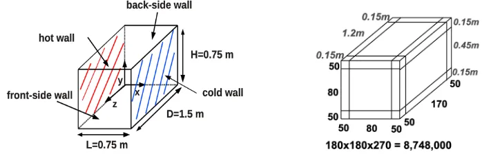
fluid exceeds a critical value of the Rayleigh-number, it starts moving, controlled by the temperature difference of the vertical, heated walls. The Prandtl number lies in this study at Pr = 0.71. The simulation assumes a non- Boussinesq fluid, consequently, temperature dependent fluid properties are calculated by the Sutherland model as stated in [2]. The computational geometry consists of a Cartesian block-structured mesh with 27 blocks. A scheme of the mesh can be seen in Figure 1, right picture. This mesh partition enables an exterior zone where a finer resolution can easily be chosen independently of the other blocks. Directly at the walls the mesh is clus- tered and the cell ratios decrease to the walls. In this way, all relevant turbulent scales can be resolved and no wall functions have to be considered. In the middle of the geometry, large scales of the flow are dominant. Thus, the mesh can have a coarser resolution in this region than close to the walls. The final mesh consists of
(180 180 270)× × =8, 748, 000 cells in (x,y,z)-direction. The first grid point is located at 4 1 5 10 m w
y = × − in vertical distance to the hot, respectively cold, wall. To analyse possible grid dependencies, additionally to the 3D simulation also a 2D simulation is performed with a mesh resolution of
(
750 750×)
=562, 500 cells in (x,y)-direction. The cells are equally spaced over the plane. The first grid point is located at 41 6.9 10 m w
y = × −
in vertical distance to the hot, respectively cold, wall. The non-dimensional distance from the wall y+ is given by
0
1 with u and ,
y
w
u y
u
y
υ
τ y ττ
ρωτ
ωµ
=
+ ∂
∂
= = = (2)
where uτ is the wall shear rate, υ the kinematic viscosity and
µ
dynamic viscosity.0
/
y
u y
=
∂ ∂ marks the
velocity gradient directly at the wall. Table 1lists values of y+ estimated in the first cell midpoint yw1 in the
full turbulent flow for both simulation types and both temperature boundary conditions.
The different values between the simulation types are caused by different velocities close to the heated walls.
3. Governing Equations
[image:3.595.91.539.257.305.2]
Figure 1. Left: Configuration of the computational test case. Right: Computational mesh resolu- tion with
(
180 180 270× ×)
=8,748,000 cells.Table 1. Temperature boundary conditions and values of the non-dimensional wall distance y+.
Boundary condition 3D 2D
Adiabtic y+=0.112 y+=0.0482
Linear temperature y+=0.332 y+=0.190
simulation tool OpenFOAM®. In a LES the flow is separated in large and small scales, the so-called subgrid scales (marked by index “sgs” in the following). The large scales are solved directly on the discretisation grid, while the subgrid scales are modelled with an applicable turbulence model, which is in this study the so-called model of Fureby [3]. This model is based on the compressible Smagorinsky model. It assumes a thermodynamic ideal gas
(
)
( )
0(
0)
1
and .
p
pM R T T h h
c
ρ = = − (3)
For the LES a space-time variable is separated and subsequent filtered as follows
( )
( ) (
)
with ,t ,t G ,t t d d .t
ψ ψ ψ ψ ∞ ∞ψ
−∞ −∞
′ ′ ′ ′
= + x =
∫ ∫
r x−r − r (4)Additionally, the dense weighted Favre-filtering of Vreman [4] is used
. ρψ ψ
ρ
=
(5)
Hence, the governing equations are
Compressible conservation of mass
( )
+ 0, t ρ ρ ∂ ∇ ⋅ =∂ u (6) Compressible conservation of momentum
(
)
( )
Tsgs
2
( ) ,
3 p
t
ρ ρ µ µ ρ
∂ + ∇ ⋅ − ∇ ⋅ + ∇ + ∇ − ∇ ⋅ = −∇ +
∂
u
uu u u u g (7)
Compressible conservation of enthalpy
( )
(
(
sgs)
)
.h p
h h p
t t
ρ ρ α α
∂ + ∇ ⋅ − ∇ ⋅ + ∇ =∂ + ⋅∇
∂ ∂
u u (8)
3 2 e ⋅ ∆
with the deviatoric part of the strain rate tensor S*ij,the filtered strain rate tensor
1 2 j i ij j i u u S x x ∂ ∂ = + ∂ ∂ (11)
and two model coefficients, ce =1.046,ck =0.02.The temperature-dependence of the fluid properties is de- scribed by the Sutherland model [2]. For ideal gases it gives a relation between the dynamic viscosity µ and the absolute temperature T
3 2 ref ref ref . S S T T T
T T T
µ µ= + +
(12)
ref
µ is a reference dynamic viscosity at a reference temperature Tref and TS is the so-called Sutherland tem- perature. In this study these coefficients are chosen as 5
ref 1.827 10 kg/ms
µ = × −
, Tref =291.15 K and
120 K. S
T =
4. Results
4.1. Temperature Profile between the Heated Walls
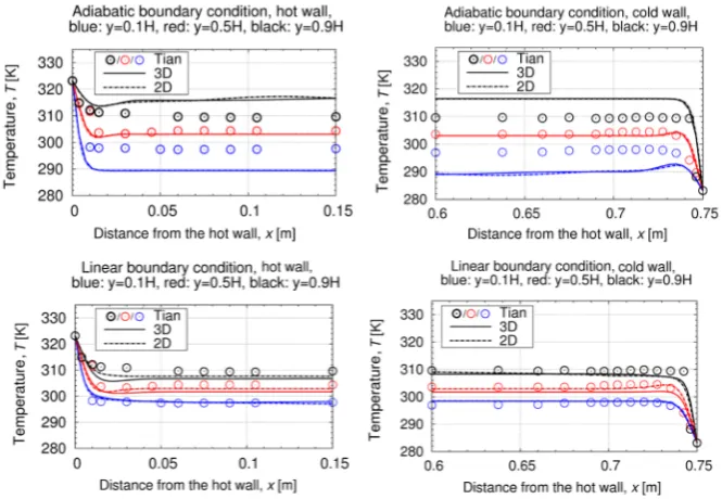
The flow movement of the convection is initialised by the temperature difference between the vertical walls. Thus, the temperature profile is one important aspect to understand the dynamic of the flow. Figure 2 displays the typical temperature and vertical velocity profile at the xy-midplane for a natural convection in the investigated setup. Near to the vertical walls, the temperature and vertical velocity can be described by a linear law. This re- gion is called the inner layer of the boundary layer. In the following, the time-averaged temperature profile is es- timated between the heated walls at the xy-midplane at x=0.75 m, z=0.75 m for three different heights,
1 0.1H, 2 0.5H and 3 0.9H
y = y = y = . The time-averaged results of the 3D and 2D simulation are plotted against the experimental data of Tian and Karayiannis [1] in Figure 3.
The thermal boundary layer near the heated walls and a variation of its thickness along the heated walls can clearly be seen. Further, a dependence on the particular boundary condition is visible. The boundary layer in- creases in the clockwise flow direction. Steep temperature gradients appear, before they reach their minimum at ca. 0.03 m afar from the hot wall (respectively 0.73 m from the cold wall), where the bulk region begins. Here, the temperature is almost stationary and almost equal to the mean temperature Tmean. The simulation profiles
Figure 2. Instantaneous temperature (left) and verticalvelocity (right) profile between the heated walls, linear temperature condition.
Figure 3. Time-averaged temperature profile at the vertical xy-midplane along the horizontal axis, at x = 0.75 m, z = 0.75 m and different heights. Top: Adiabatic bc. Bottom: Linear bc. Detailed plot of the hot/cold wall. In all pictures: y1 = 0.1H (blue), y2 = 0.5H (red) and y3 =
0.9H (black), − (solid line): 3D, − − − (dashed line): 2D. : study Tian and Karayiannis
[1], Ra = 1.58 × 10⁹.
circulation zones compared to the experiment. The 2D plot shows only slight deviations to the 3D plot. The linear results approximate the experimental data closer than the adiabatic results, due to the similar boundary condition. The results of the 2D-simulation lie even closer to the experimental data than the results of the 3D simulation.
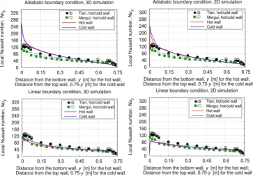
4.2. Nusselt Number Profile along the Heated Walls
[image:5.595.146.479.239.469.2]Figure 4. Time-averaged profile of the local Nusselt number along the heated walls. Top: Adiabatic bc.
Bottom: Linear bc. Left: 3D simulation. Right: 2D simulation. In each picture: − (red solid line): hot wall, − − − (blue dashed line): cold wall. Study Tian and Karayiannis [1]: ●: hot wall, : cold wall,
Ra = 1.58 × 10⁹. Study Mergui, Penot and Tuhault [12]: ∎: hot wall, □: cold wall, Ra = 1.34 × 10⁹.
3D case are slightly lower at the hot wall than at the cold one. But the values at midheight deviate in both simu- lations significantly from the data in [1], of about at most 20%. This might possibly be caused by lower tem- perature gradients. The numerical data approximate well the numerical study of Mergui, Penot and Tuhault [12].
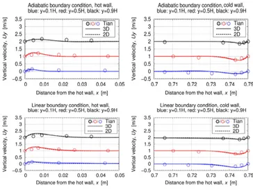
4.3. Vertical Velocity Profile between the Heated Walls
Figure 2 shows a snapshot of the instantaneous mean velocity distribution at the xy-midplane in the container
for the linear boundary condition. The plot reveals an exterior circulation zone as well as an interior one. Both circulations are reversed to each other. Furthermore, smaller circulations appear additionally in the left bottom and top right corner as well as top left and bottom right corner. In this section, the time-averaged vertical veloc- ity profile at the xy-midplane between the temperatured walls is investigated and plotted inFigure 5. The pro- files are estimated at the same positions as the temperature profiles before in Figure 3. For a better demonstra- tion a constant was added to the results of each height, which are: y1: 0, + y2: 1, + y3: 2.+
As in the temperature profile, a clockwise circulation direction and an increase of the boundary layer along the heated walls in flow direction are visible. The boundary layer reaches its maximum width at the hot wall at height y3 =0.9H (respectively at the cold wall at height y1=0.1H). The thermal boundary layer is smaller
Figure 5. Time-averaged vertical velocity profile at the xy-midplane, at x = 0.75 m, z = 0.75 m and different heights. Top: Adiabatic bc. Bottom: Linear bc. Detailed plot of the hot/cold wall. In all pictures: y1 = 0.1H (blue), y2 = 0.5H (red) and y3 = 0.9H (black), − (solid line): 3D, − − − (dashed line):
2D. : study Tian and Karayiannis [1], Ra = 1.58 × 10⁹.
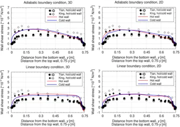
4.4. Wall Shear Stress along the Heated Walls
According to Tian and Karayiannis in [1], a cubic law can be assumed for the velocity profile in the outer re- gion of the inner layer. Therefore, the shear stress profile is described as
[ ]
2, N/m ,
y
w w
w u
x
τ =µ∂ τ =
∂ (13)
with the gradient of the vertical velocity component directly at the heated walls (index w) and a depending dy- namic viscosity µ. Besides the experimental data of [1] also another experimental study of King [13] is com- pared to the numerical data of this study in Figure 6.
As Figure 6 shows, the time-averaged shear stress rises, analogously to the velocity, along the vertical, heated
walls to its peak value and back to zero in the corners. The results of [1] reveal an asymmetry in the corner re- gions. The data of King [13] reveals higher values than in the study of Tian and Karayiannis [1], which are pos- sibly caused by a higher investigated Rayleigh number of King [13] according to [1]. The simulation profiles show an asymmetrical form, which is founded in the asymmetrical velocity profile.All simulations reveal nega- tive values in the top hot and bottom cold corner which indicate anti-clockwise vortex regions as mentioned in [1]. The values along the heated walls in this study are higher than the data of [1], due to higher velocity gra- dients and higher dynamic viscosity values. The high values of this study approximate rather the data of King [13] than of Tian and Karayiannis [1].
5. Conclusion
[image:7.595.130.494.83.357.2]Figure 6. Time-averaged wall shear stress profile along the heated walls. Top: Adiabatic bc. Bottom:
Linear bc. Left: 3D simulation. Right: 2D simulation. In all pictures: − (red solid line): hot wall, − (blue solid line): cold wall. Study Tian and Karayiannis [1]: •: hot wall, : cold wall, Ra = 1.58 ×
109. Study King [13]: ♦: hot wall, ◊: cold wall, Ra = 4.5 × 10⁹.
2-dimensional simulations were executed to investigate possible grid dependencies. Taking the different boun- dary conditions and the non-Boussinesq fluid assumption of the computational study into consideration, the re- sults of the investigated fluid properties in all 3-dimensional simulations approximated well the experimental results of [1]. The simulation data showed the same profile tendencies as in the experiment [1]. The results of the 2- and 3-dimensional simulations revealed in most cases similar results and only small deviations to each other which appeared mainly in vicinity to the heated walls. These deviations have to be further investigated in future studies to find an additional explanation as the one of grid dependencies. Summarising, the presented LES is very qualified to model the flow structures and fluid properties profiles of a turbulent, natural convection flow in the investigated configuration of a rectangular container where the vertical walls are heated.
Acknowledgements
The authors wish to thank the North-German Supercomputing Alliance (HLRN) for providing their hardware during the numerical simulations of this study.
References
[1] Tian, Y.S. and Karayiannis, T.G. (2000) Low Turbulence Natural Convection in an Air Filled Square Cavity, Part I: The Thermal and Fluid Flow Fields. International Journal of Heat and Mass Transfer, 43, 849-866.
http://dx.doi.org/10.1016/S0017-9310(99)00199-4
[2] Sutherland, W. (1893) The Viscosity of Gases and Molecular Force. Philosophical Magazine, Series 5, 36, 507-531.
http://dx.doi.org/10.1080/14786449308620508
[3] Fureby, C. (1996) On Subgrid Scale Modeling in Large Eddy Simulations of Compressible Fluid Flow. Physics of Fluids, 8, 1301-1311. http://dx.doi.org/10.1063/1.868900
[4] Vreman, B. (1995) Direct and Large-Eddy Simulation of the Compressible Turbulent Mixing Layer. Ph.D. Thesis, University of Twente, Enschede.
[6] Sergent, A., Joubert, P. and Quéré, P. Le (2003) Development of a Local Subgrid Diffusivity Model for Large-Eddy Simulation of Buoyancy Driven Flows: Application to a Square Differentially Heated Cavity. Numerical Heat Transfer,
Part A: Applications, 44, 789-810.
[7] Shishkina, O. and Wagner, C. (2008) Analysis of Sheet-Like Thermal Plumes in Turbulent Rayleigh-Bénard Convec- tion. Journal of Fluid Mechanics, 599, 383-404. http://dx.doi.org/10.1017/S002211200800013X
[8] Shishkina, O. and Thess, A. (2009) Mean Temperature Profiles in Turbulent Rayleigh-Bénard Convection of Water.
Journal of Fluid Mechanics, 633, 449-460. http://dx.doi.org/10.1017/S0022112009990528
[9] Kosović, B., Pullin, D.I. and Samtaney, R. (2002) Subgrid-Scale Modeling for Large-Eddy Simulations of Compressi- ble Turbulence, Physics of Fluids, 14, 1511-1522. http://dx.doi.org/10.1063/1.1458006
[10] Erlebacher, G., Hussaini, M.Y., Speziale, C.G. and Zang, T.A. (1992) Toward the Large-Eddy Simulation of Compres- sible Turbulent Flows. Journal of Fluid Mechanics, 238, 155-185. http://dx.doi.org/10.1017/S0022112092001678
[11] Gifford, W.A. (1991) Natural Convection in a Square Cavity without the Boussinesq-Approximation. 49th Annual Technical Conference-ANTEC’91, Montreal, 5-9 May 1991, 2448-2454.
[12] Mergui, S., Penot, F. and Tuhault, J.H. (1993) Experimental Natural Convection in an Air-Filled Square Cavity at
9
Ra=1.7 10⋅ . In: Henkes, R.A.W.M. and Hoogendoorn, C.J., Eds., Turbulent Natural Convection in Enclosures—A Computational and Experimental Benchmark Study, Proceedings of the Eurotherm Seminar no 22, Editions Europé- ennes Thermique et Industrie, Paris, 9-108.