Application of Genetic Algorithm in Power System
Optimization with Multi-type FACTS
Nadil Amin
1, Abu Qauser Marowan
2, Bashudeb Chandra Ghosh
31,2
Department of Electrical Engineering, The University of Sydney
3
Department of EEE, Khulna University of Engineering & Technology
1
Email: [email protected]
Abstract- In this era of energy crisis, the power system operators are very much driven to minimize the overall system loss and generation cost. Maximization of network load-ability without compromising the system stability has become a major concern for them. Introduction of FACTS technology can help a system to achieve these goals without building new transmission lines that is both expensive and time consuming. However, the new installation of FACTS in the system has to be optimal in terms of its type, location and size. This paper seeks to present a genetic algorithm based framework that can optimize a system having FACTS devices with an objective of improved economic dispatch. The IEEE 14 & 30 bus systems are taken as illustrative examples to validate the effectiveness of proposed method.
Index Terms- FACTS, Genetic Algorithm, Optimization, Load-ability, Economic Dispatch.
I. INTRODUCTION
Problem Statement
The deregulated market model is progressively taking place in power industries all over the world. With such liberalization, a third-party access is provided by separating the generation & transmission of power, and the consumers are empowered to pick from the private utilities as per their own choices for the electricity-buying purpose. However, in order to grab a larger customer-base and survive in the market, these suppliers might cause the commercial rivalry to take an unhealthy turn and resort to the unplanned power exchange through transmission lines. Parallel to restructuring of market, the industry also faces the challenge of satisfying the ever-increasing growth of load demand. All these force to operate some of the transmission lines close to their thermal limits which could result in being overstressed and eventually in congestion. On the other hand, the up gradation of power network by building new infrastructures like transmission lines, substations etc, most of the time, turns out to be not practical due to political, economical & environmental constraints.
Therefore, the general consensus is to have a better utilization of existing network by making it more smart, fault tolerant and self healing. Such maximization of network’s power flow efficiency in terms of decreasing overall loss, cost & instability threats could be realized by introducing power electronics applications like FACTS devices (Flexible Alternating Current Transmission Systems). Proposed by N. Hingorani [1]; this advanced
semiconductor technology can provide technical solution to address the following operating challenges, and enhances the useable capacity limits of existing transmission lines by means of numerous control functions like voltage regulation, active-reactive power control, system damping etc, in a fast & effective manner.
Nevertheless, there are various types of FACTS and each type has got its own advantages to achieve a specific goal. Thus the most effective use of FACTS largely depends on whether a suitable type is used in a defined context or not. Moreover, the high investment cost drives the device to be installed optimally in the system rather than arbitrarily. Therefore, the new installation of FACTS must be well-planned in terms of its type, location & rating, and requires an assessment of power system efficiency through off-line simulations. This paper is concerned about developing a robust algorithm which can optimize a system with FACTS devices such that the system load-ability can be increased as much as possible at minimum cost.
FACTS Device Generalities
We know, the power flow in an interconnected network can be represented by the following two relationships.
𝑃𝑖𝑗 =
𝑉𝑖𝑉𝑗
𝑋𝑖𝑗
sin 𝛿𝑖𝑗 & 𝑄𝑖𝑗=
1 𝑋𝑖𝑗
(𝑉𝑖2− 𝑉𝑖𝑉𝑗cos 𝛿𝑖𝑗)
FACTS technology has also got several other devices that fall into different categories and are developed to serve different purposes. These are not reported here for the sake of length of paper.
Simulation Tools & Test Bed System
The IEEE benchmark systems of 14-bus and 30-bus are selected as test bed systems for the simulation of the following research. To carry out the optimization process, an algorithm code is written in visual C++ language. The code is then applied on the system to solve power flow problem with the help of a Matlab based power simulation package called Matpower 4.1 [2].
Scope of Genetic Algorithm
As it is known by now that optimal allocation of FACTS is a nonlinear complex problem that involves combinatorial analyses. The inclusion of multiple objectives, existence of both discrete (i.e. locations & types) & continuous (i.e. ratings) domain variables, and apprehension of getting stuck at any of the several local minima available in the search space, etc - all make the problem such complicated that a well-efficient heuristic method like Genetic Algorithm should be employed to solve it in a reasonable computation time. GA is a parallel and global search technique that was developed by J. Holland on the basis of Darwin’s survival of the fittest theory. This technique is ‘intelligent’ in finding optimality since it can evaluate many points simultaneously in the search space, and emulates ‘human reasoning’ while moving from one solution point to other.
II. PROBLEMFORMULATION
Objective Function
The aim of research is that to increase the system load-ability as much as possible in both steady and transient states of operation by utilizing the maximum benefits of FACTS at minimum cost. Nevertheless, the optimal amount of power flow has to be achieved without compromising any of the network constraints such as bus voltage deviation level, thermal limit of transmission line etc. All these requirements make the allocation of FACTS device a multi-objective optimization problem which involves a non-linear complex formulation comprised of both integer and continuous variables. Mathematically, the following OPF problem can be formulated using an economic saving function that incorporates the generation cost along with the FACTS installation cost as being subjected to the constraints mentioned below.
The first function that deals with the operating cost of generation units in system can be written as a quadratic polynomial:
𝐶𝐺𝑒𝑛 = ∑ 𝐶𝑖(𝑃𝐺 𝑖) 𝑖=𝑁𝐺
𝑖=1
𝐶𝑖(𝑃𝐺 𝑖) = 𝑎𝑖𝑃𝐺 𝑖2+ 𝑏𝑖𝑃𝐺 𝑖+ 𝑐𝑖 ($/ℎ𝑟)
where, 𝑎𝑖, 𝑏𝑖, 𝑐𝑖 are the generation cost coefficients that represents the measure of loss, fuel cost and other expenses like wages, interest etc respectively. 𝑃𝐺 𝑖 simply denotes to the real power generation of i-th generator whereas NG is the total number of units in the system.
The second cost function is developed from the database of Siemens AG [3] to take the investment on FACTS into account.
Such investment includes equipment cost, infrastructure cost and site civil works etc.
𝐶𝐹𝐴𝐶𝑇𝑆= ∑ 𝐶𝑗(𝑆𝑗)
= ∑[𝑆𝑗2𝛼𝐹𝑡𝑦𝑝𝑒+ 𝑆𝑗𝛽𝐹𝑡𝑦𝑝𝑒+ 𝛾𝐹𝑡𝑦𝑝𝑒] ($/𝐾𝑉𝐴𝑟)
Here, 𝛼, 𝛽 & 𝛿 are FACTS cost coefficients that differ with the types of FACTS devices (i.e. Ftype = TCSC, SVC, UPFC etc). 𝑆𝑗 is the operating range of FACTS at j-th location in MVAr. It is basically the difference between reactive power flows before & after inserting the device in the transmission line.
𝑆𝑗 = |𝑄2𝑗− 𝑄1𝑗|
All the parameter values that involve in these two cost functions are provided in Appendix. The objective function is then determined by adding these functions together. However, before merging the 2 equations, the unit of FACTS cost function also needs to be converted to ($/ℎ𝑟).
𝐶′𝐹𝐴𝐶𝑇𝑆=
𝐶𝐹𝐴𝐶𝑇𝑆× 𝑅𝐹𝐴𝐶𝑇𝑆× 1000
8760 × 5 ($/ℎ𝑟)
The following unit conversion formula includes 5 years to be considered as the average device lifetime. This value is selected randomly and does not have any influence on the optimization process as it is applied only to unify the unit. However, technically, FACTS can serve even more than 5 years [4, 5]. Thus the optimization objective becomes as to
𝑚𝑖𝑛𝑖𝑚𝑖𝑧𝑒, 𝐶𝑇𝑜𝑡𝑎𝑙= 𝐶𝐺𝑒𝑛+ 𝐶′𝐹𝐴𝐶𝑇𝑆
Fitness Function
Fitness is a scalar measure of quality that helps in assessing the solutions available in the problem hyperspace and distinguish the most promising ones. It is formed on the basis of objective function. Now genetic algorithm works better in solving the maximization problems rather than the minimization ones as it emulates the nature’s ‘survival of fittest’ principle. Hence, the following minimization problem is transformed into a maximization one by adopting the fitness function stated below.
𝑌 = 𝑚𝐶𝑇𝑜𝑡𝑎𝑙+ 𝑁
where, m is a scaling factor which is equal to -1 to convert the minimization problem and N is a large positive constant to offset the fitness value from being negative. Moreover, in order to avoid slow convergence of algorithm by emphasizing the best solutions in the pool, the ultimate fitness function is derived such that it is normalized into the range 0 to 1.
𝐹 = 1
1 + 1 𝑌⁄ =
𝑁 − 𝐶𝑇𝑜𝑡𝑎𝑙
𝑁 − 𝐶𝑇𝑜𝑡𝑎𝑙+ 1
Search Space Constraints
The optimization problem is subjected by several constraints that can be categorized broadly into two classes named as equality and inequality constraints. The first of them arises out of the necessity of balancing real and reactive power generation in the system, while the second type characterizes the physical and operational limits of network components along with FACTS devices. Each constraint puts a limit in the search domain and must be satisfied by the solutions in order to be considered as feasible. The solutions that lie beyond these limit-boundaries are infeasible and discarded without having any fitness test.
margin. Nonetheless, the integration has to be well planned by limiting the number of devices to a certain level so that the new investment required for device-integration remain convenient. Thus the constraint is defined such that a particular solution can recommend to install maximum 4 devices at a time in the system.
0 ≤ 𝑁𝐹𝐴𝐶𝑇𝑆 ≤ 4
Constraint: Types of Device: As it is mentioned before, several FACTS devices has been developed thus far, and it is not practical to incorporate all the technologies in this optimization problem. Depending on the types of compensation, the following research has taken TCSC, SVC and UPFC into consideration. TCSC is selected from the series controller group whereas SVC is a shunt controller. UPFC has got the combination of both series & shunt connections.
Constraint- Possible Location of Device: All the FACTS except SVC can directly be inserted into the transmission lines of the system. The SVC has to be connected at sending bus node, receiving bus or at middle point of line by splitting it into 2 equal parts. Moreover, the generator buses do not need any FACTS and can be omitted from the search space. It is because the voltages of these buses will be regulated automatically by the corresponding generators’ AVRs. For example, there are 20 transmission lines and 9 PQ buses in the selected 14 bus system. Hence, the following constraint for this system can be defined as-
1 ≤ 𝜆𝑇𝐶𝑆𝐶≤ 20; 1 ≤ 𝜆𝑈𝑃𝐹𝐶 ≤ 20; 1 ≤ 𝜆𝑆𝑉𝐶≤ 9 (1)
Constraint- No. of Device per Line: A particular transmission line should not be occupied by more than 1 FACTS at a time since it will hamper each other’s performance that leads to none of the device working properly [6].
𝜆𝑖≠ 𝜆𝑗 ∀𝑖, 𝑗 (2)
Constraint- Size of Device: The ratings of selected FACTS devices need to be suitable for the steady state operation of the test system. For example, in order to avoid the overcompensation of transmission line, TCSC is permitted to modify the line reactance up to |0.2𝑋𝑙𝑖𝑛𝑒| in inductive mode and |0.7𝑋𝑙𝑖𝑛𝑒| in capacitive mode. Similarly, the chosen UPFC can inject maximum 10% of the line voltage by varying its phase angle from -180 to +180. Finally, a SVC is allowed to absorb or supply maximum 100MVAr reactive power in the system.
−0.7𝑋𝑙𝑖𝑛𝑒≤ 𝑅𝑇𝐶𝑆𝐶≤ 0.2𝑋𝑙𝑖𝑛𝑒;
−180° ≤ 𝑅𝑈𝑃𝐹𝐶 ≤ 180°;
−100𝑀𝑉𝐴𝑟 ≤ 𝑅𝑆𝑉𝐶≤ 100𝑀𝑉𝐴𝑟
Constraint- System Power Balance: It is an equality constraint that is imposed on network model to maintain a power balance such that the total load demand and transmission loss must be equal to the active power generated by the online units at each time interval.
∑ 𝑃𝐺 𝑖
𝑁𝐺
𝑖=1
= 𝑃𝐷𝑒𝑚𝑎𝑛𝑑+ 𝑃𝐿𝑜𝑠𝑠
Constraint- Generator Operational Limit: It is well known that the prime mover imposes maximum & minimum limits on the active power output of a generator. Similarly, the reactive power capability of generator is also constrained as a function of its active power generation. No unit should be dispatched beyond
these permissible ranges as given in appendix for the purposes of safety and economy.
𝑃𝑖𝑚𝑖𝑛≤ 𝑃𝐺 𝑖≤ 𝑃𝑖𝑚𝑎𝑥; 𝑄𝑖 𝑚𝑖𝑛≤ 𝑄𝐺 𝑖≤ 𝑄𝑖 𝑚𝑎𝑥
Constraint- Bus Voltages: Theoretically, the voltage desired at each bus is 1pu. However, practically it never be equals to unity and is permitted to deviate within ±5% of the nominal value.
0.95𝑝𝑢 ≤ 𝑉𝑖≤ 1.05𝑝𝑢; 𝑖 = 1,2, … , 𝑁𝑏𝑢𝑠
III. ALGORITHMIMPLEMENTATION
Encoding
The implementation of a genetic algorithm initiates by encoding the parameters of the optimization problem into chromosomes (individuals). A chromosome is typically a string which will represent one of many feasible solutions to the problem in the search space. It is very necessary to encode the parameters carefully so that the developed algorithm is able to transfer information between the chromosomes and the objective function efficiently. The elements of a chromosome could be binary bits, real numbers or even other cardinality alphabets. In the following algorithm, binary coded strings are used to represent the chromosomes. Since binary representation has got the minimum no. of alphabets (only 0s & 1s), the manipulation of these binary strings by GA operators become easier.
According to our search space constraints, we can install maximum 4 FACTS devices in the test system, which means each chromosome (solution) consists of 4 strings where each string carries information about a particular FACTS device. Since the configuration of FACTS devices in our case is defined with three parameters such as types, locations & ratings, each string gets three subsets of binary representations. Here, the 1st subset of a string indicate the location of a FACTS, whereas the 2nd & 3rd subsets correspond to its type and rating respectively. Since there are maximum 20 possible locations in the system for installing FACTS (equation 1) and 24< 20 < 25, the number of bits in the 1st subset should be 5. Again, the 3 types of FACTS devices that are taken into consideration to improve the performance of the power system could be encoded as follows: ‘1’ for TCSC, ‘2’ for SVC, & ‘3’ for UPFC. However, a 4th
case is also possible which depicts the situation of ‘no FACTS required’, This 4th type of case can also be denoted by some
value such as ‘0’. This means we need 2 bits in the 2nd subset to
represent the parameter of FACTS-types.
Finally, similar rule (mentioned in equation 3) can also be used to determine the number of bits required for the last subset, which is 8. However, before that, the different ranges of FACTS ratings need to be normalized into a common range, such as -1 to +1. This helps the encoding & decoding of binary strings to be easier.
2𝑙≥ (𝑥𝑚𝑎𝑥− 𝑥𝑚𝑖𝑛
∆𝑥 + 1) (3)
𝑤ℎ𝑒𝑟𝑒 𝑙 𝑖𝑠 𝑡ℎ𝑒 𝑠𝑡𝑟𝑖𝑛𝑔 𝑙𝑒𝑛𝑔𝑡ℎ 𝑡𝑜 𝑝𝑟𝑜𝑣𝑖𝑑𝑒 ∆𝑥 𝑣𝑎𝑟𝑖𝑎𝑡𝑖𝑜𝑛 𝑖𝑛 𝑎𝑐𝑐𝑢𝑟𝑎𝑐𝑦
𝑅𝑛 𝑇𝐶𝑆𝐶=𝑅𝑇𝐶𝑆𝐶+ 0.25
0.45 ; 𝑅𝑛𝑆𝑉𝐶=
𝑅𝑆𝑉𝐶
100; 𝑅𝑛𝑈𝑃𝐹𝐶= 𝑅𝑈𝑃𝐹𝐶
180
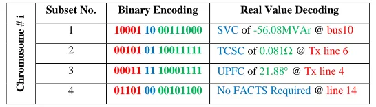
absorb 56.08MVar reactive power with a SVC at bus 10; shift phase angle by 21.88 through an UPFC at transmission line 4; and change reactance of line 6 by 0.081 with a TCSC.
Table I: Representation of FACTS configuration by binary coded string
C
h
ro
m
o
so
m
e
#
i Subset No. Binary Encoding Real Value Decoding
1 10001 10 00111000 SVCof -56.08MVAr @ bus10 2 00101 01 10011111 TCSC of 0.081@ Tx line 6 3 00011 11 10001111 UPFC of 21.88 @ Tx line 4 4 01101 00 00101100 No FACTS Required @ line 14 Initial Population
Using the strategy described above, an N number of individuals are encoded which comply with all the search space constraints. This set of N individuals is regarded as the 1st population set which will evolve from generation to generation with a hope of creating more suitable individuals in future, and eventually converging into a global optimum solution. The advantage of genetic algorithm is that it is not so sensitive to such starting points of the search process for optimum solution. An initial chromosome can be formed by flipping an unbiased coin which has a probability of 0.5. For example, in our case, the coin has to be tossed 60 times in order to get a 60 bits long chromosome. This can be done by calling a random number generating function such as ‘rand’ 60 times in the algorithm code with the help of ‘for’ loop.
However, some care has to be taken while using the loop. For example, the 5 bits allocated for ‘FACTS location’ can produce
25= 32 different values, whereas we have maximum 20 installation sites in the 14 bus system. Thus the algorithm is coded to discard the other 12 values if generated, which can not be assigned to any of these 20 locations. In addition, if a SVC related chromosome includes a generator bus as its location, the location will be changed to the closest load bus (constraint presented in equation 1). Moreover, since a particular transmission line could have only one FACTS at a time (equation 2), each location can appear maximum once in the string of a chromosome, and the later location will be re-randomized if repeated. Lastly, the algorithm is also programmed to discard any identical chromosome that appears twice in the population set. In this way, the entire set of initial population is obtained by repeating the above steps N=20 times as we set there will be 20 individuals born in each generation.
Once the entire population is formed, the real values of parameters are decoded from the binary strings, and introduced in the test system to evaluate the FACTS impacts on the state of power system by invoking Matpower solver. Finally, the fitness of each individual is measured by employing the power flow outputs in the fitness function defined in section II.
Selection
The GA solver keeps expanding its search space by incorporating more and more solutions evolved from the above set of ancestors until a stopping criterion is met. The future offspring will be bred out of a mating pool formed by the fitter candidates of the antecedent population set since the algorithm is inspired by Darwin’s “survival of the fittest” concept. It is a common phenomenon of biological evolution process seen in nature such that the fitter creatures are more likely to survive the competition
by yielding better genetic inheritance. Thus the better fitness an individual possesses, the more chance it has to be selected as genitor in the pool. There are a number of ways that the selection scheme can be implemented in algorithmic form such as Roulette wheel selection, rank selection, Boltzmann selection, steady state selection, tournament selection etc.
This paper adopts the Roulette wheel technique to accomplish the fittest test. To do so, the algorithm is first coded to compute the cumulative probability for each of the 20 individuals by successively adding their probabilities from top to bottom of the current population set. That means the bottom most individual in the set will get a cumulative probability equal to 1.0. Then a random number is let to be generated between 0 to 1, and the individual will be selected according to the range the generated number falls into. This is repeated for 20 times to form the complete mating pool. For example, an i-th chromosome is
expected to make 𝐹𝑖𝑡𝑛𝑒𝑠𝑠𝑖
𝐹𝑖𝑡𝑛𝑒𝑠𝑠𝑎𝑣𝑔 copies in the pool. The whole process actually mimics the roulette wheel game- ‘All we have to do is spin the ball and grab the individual at the point it stops’. The higher fitness an individual has, the wider area it will occupy in the wheel’s circumference and the more chances the pointer will get to be in that area.
Crossover
After the mating couples are decided, a genetic operator called crossover is employed to inherit the DNA information from the parental genes and rearrange them to produce new offspring solutions for the next population set. The type of such genetic operation could be single, double or uniform depending on the nature of decomposition and recombination. In a double crossover, which is our case, two uniform cross-sites are chosen randomly along the strings of parent individuals. The bits in one parent-individual before & after these cut-points are classified into separate groups, and exchanged with the corresponding groups of the other parent-individual. However, the two cross-sites can not be located at any arbitrary bit-position in the string. Since the representation of any single device needs a distinct substring of 15 bits, and no decomposition can be done in such a unit domain, the two cross-sites must be defined in the algorithm as
𝐾1∈ {1, 16, 31, 46}
𝐾2∈ {16, 31, 46, 60}
& 𝐾1≠ 𝐾2
Now if (𝐾1, 𝐾2) = (16,45) is selected for a particular couple, then they will swap the 2nd & 3rd substrings between them while keeping the other 2 substrings unchanged in order to generate new solutions (Table- II).
Table II: Two point crossover operation
Parent Chromosome 1 100011000111000 001010110011111 000111110001111 011010000101100
Parent Chromosome 2 101011001011000 100111010011011 010100101101111 001011100110100
Offspring Chromosome 1 100011000111000 100111010011011 010100101101111 011010000101100
Offspring Chromosome 2 101011001011000 001010110011111 000111110001111 001011100110100
Table III: Correction process: rearrangement of FACTS
Offspring Chromosome 1 (No Correction) 100011000111000 100111010011011 010100101101111 011010000101100
Offspring Chromosome 2 (Before Correction) 101011001011000 001010110011111 000111110001111 001011100110100 (After Correction) 101011001011000 011010110011111 000111110001111 001011100110100
Table IV: Operation of mutation
Offspring Chromosome i
(Before Mutation) 101011001011000 011010110011111 000111110001111 001011100110100
(After Mutation) 101011001011000 010010110001111 000110110001111 001011100110100
The following algorithm lets the crossover operation to take place with a high probability of 𝜌𝑐= 0.9. That means there is a certain rate of 10% where no crossover will be performed, and off-spring will be an exact copy of its parents.
The new off-springs are usually expected to be even more novel solutions as they are formed by combining the good substrings from their father and mother nodes who have already passed the competitive selection process. The only matter that needs to be considered here is whether or not an appropriate cross-site is selected. Nevertheless, if good solutions are generated by crossing over, there will be more copies of them in the next mating pool. If good strings are not formed, then they will die out eventually in the subsequent generations through the selection operator. In this way, the algorithm will gradually proceed to find out the optimum solution point.
Mutation
After crossover, the newly created individuals sometimes need to undergo the process of mutation. This is required since the new generation nodes might not carry any significant new inheritance information which can lead to a problem of all solutions falling into a local optimum point instead of the global optimum. Population diversity is very much required to search a big part of the search space and incorporate the regions not viewed before by the algorithm.
Mutation operator comes occasionally in action with a low probability of 0.05 ~ 0.1, and alters the bits selected randomly in a string, that is changing ‘0’ to ‘1’ & vice versa. In our case, we let all the four substrings of an individual to be mutated independently and draw new values from the possible set of their parameters. For example, the 2nd & 3rd strings of a random i-th chromosome can be selected for mutation where bit no. 18, 26 & 36 will be altered to add new information to the population (Table-IV).
Termination
The newly generated solutions are then reintroduced in the test system for power flow analysis and ranked again according to their fitness behaviour. The new mating pool then comprises of the best solutions generated thus far including both parents and off-springs. So the average fitness of the population will either increase or remain same for the new generation than the previous
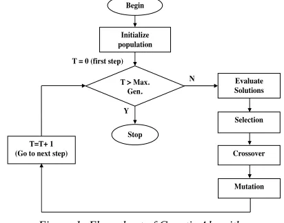
[image:5.612.340.546.411.573.2]one. In this way, the algorithm applies the stochastic operators like selection, crossover, mutation etc iteratively to grow the population and completes its ‘exhaustive’ search process. Furthermore, to guarantee the movement all particles over the feasible region, the constraints of section II are applied simultaneously. The generational process continues to repeat until the algorithm converges to a solution that is the global optimum or meets the confidence threshold set by the user. Such threshold could be any fixed number of generations, any high fitness value that has reached a plateau or even exceeding any allocated budget such as computation time etc. The flow chart in figure- 1 depicts how the algorithm processes data step by step.
Figure 1: Flow chart of Genetic Algorithm
IV. RESULTANALYSIS
generation (Table- V). The active and reactive power losses will be reduced by 80kW and 220kVAr accordingly. Moreover, the voltage profile also gets enhanced and remains close to unity (Figure- 3). All of these improvements will fortify the load-ability and security of the system.
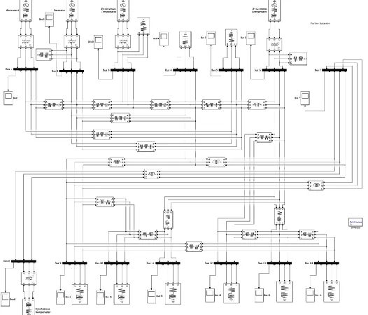
[image:6.612.37.300.117.342.2]Figure 2: Simulink model of IEEE 14 bus system
Figure 3: Voltage profile enhancement due to optimization
[image:6.612.73.261.354.529.2]Figure 4: FACTS Cost Functions
Table V: Power flow results of IEEE 14 bus system
System Parameter Before
Optimization
After Optimization Total Generation Capacity 772.4 MW 772.4 MW
Load Demand 259 MW 259 MW
Total Power Generated 272.39 MW 272.31 MW Total Active Loss 13.393 MW 13.313 MW Total Reactive Loss 54.54 MVAr 54.32 MVAr Generation Cost ($/MW-hr) 29.99964 29.99670
Maximum Branch Loss 4.30 MW @line1-2
4.26 MW @line1-2
The optimization technique did not prefer UPFC over SVC to address the problem even though the former one is the most powerful & versatile FACTS technology. It was well expected since the objective here was defined in terms of economic criteria, and UPFC is the most expensive device among the three [Figure- 4]. The high accuracy level of controlling power and relatively lower cost made SVC the most convenient solution in this case.
An Ant Colony Optimization technique has been reported in [8] to solve the same optimization problem regarding the same 14 bus system. However, the current paper’s approach turns out to be more successful in attaining optimality. It is certain that the improvements that were brought in generation cost reduction & system performance are same in both the papers (i.e. if the values were not rounded). Nevertheless, to do so, the device suggestion in [8] would ask for more FACTS-investment, and eventually longer payback period. For example, in order to bring the following improvements, our suggested solution will cost the system $75.47/hr in a time period of 5 years whereas in case of [8], it is about $76.98/hr. This reinforces our claim about the robustness of genetic algorithm that if the parameters are well tuned in the algorithm, then GA can also solve combinatorial problems efficiently just like other heuristic methods such as PSO, ACO etc.
An optimization is also carried out on the IEEE 30 bus system with the data presented in appendix. The result shows that the optimal configuration of FACTS for this system should be an SVC of 50.06MVar at bus no. 8. With such FACTS allocation, the system loss and generation cost can be minimized by 10.48% and $0.76/hr accordingly (Table- VI).
Table VI: Power flow results of IEEE 30 bus system
System Parameter Before
Optimization
After Optimization Total Generation Capacity 335 MW 335MW
Load Demand 189.2 MW 189.2 MW
Total Power Generated 191.6 MW 191.4 MW
Total Active Loss 2.448 MW 2.188 MW
Total Reactive Loss 8.99 MVAr 7.95 MVAr Generation Cost 593.441 $/hr 592.682 $/hr Maximum Branch Loss 0.29 MW
@line2-6
0.25 MW @line2-6
0 2 4 6 8 10 12 14
Bus no.
0 0.2 0.4 0.6 0.8 1 1.2
V
o
lt
a
g
e
(
p
u
)
Voltage Profile of IEEE 14 Bus System After Optimization
[image:6.612.67.268.550.721.2] [image:6.612.311.580.571.692.2]V. CONCLUSION
This work has sought to answer several questions on the behavior of genetic algorithm in solving real world problems like optimal allocation of FACTS devices. The simulation result certifies that the setting of various control parameters such as fitness formulation, selection criteria, mechanisms of crossing over & mutation etc have a strong bearing on the robustness of algorithm.
[image:7.612.34.360.191.553.2]APPENDICES
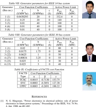
Table VII: Generator parameters for IEEE 14 bus system
Generator (Bus no.)
Cost Function Coefficients Active Power Limit a
($/MW2hr)
b ($/MWhr)
c ($)
Pmax
(MW)
Pmin
(MW) 1 (1) 0.0430293 20 0 332.4 0
2 (2) 0.25 20 0 140 0
3 (3) 0.01 40 0 100 0
4 (6) 0.01 40 0 100 0
5 (8) 0.01 40 0 100 0
Table VIII: Generator parameters for IEEE 30 bus system
Generator (Bus no.)
Cost Function Coefficients Active Power Limit a
($/MW2hr)
b ($/MWhr)
c ($)
Pmax
(MW)
Pmin
(MW)
1 (1) 0.02 2 0 80 0
2 (2) 0.0175 1.75 0 80 0
3 (22) 0.0625 1 0 50 0
4 (27) 0.00834 3.25 0 55 0
5 (23) 0.025 3 0 30 0
6 (13) 0.025 3 0 40 0
Table IX: Coefficients of FACTS cost Function
FACTS Type
Cost Function Coefficients
α β γ
TCSC 0.0015 -0.7130 153.75 SVC 0.0003 -0.3051 127.38 UPFC 0.0003 -0.2691 188.22
REFERENCES
[1] N. G. Hingorani, “Power electronics in electrical utilities: role of power electronics in future power systems,” Proceedings of the IEEE, Vol. 76 No. 4, Apr. 1988, pp.481-482.
[2] Ray D. Zimmerman and E. Carlos Murillo-Sanchez, “Matpower A MatlabTM Power System Simulation Package Version 4.1,” User's Manual, Jun. 2012.
[3] K. Habur and D. Oleary, “FACTS- flexible AC transmission system for cost effective and reliable transmission of electrical energy,” Siemens, 2004. [4] N. G. Hingorani, L. Gyugyi, “Understanding FACTS – Concepts and
technology of Flexible AC Transmission Systems,” IEEE Press, 2000. ISBN 0-7803-3455-8.
[5] F. D. Galiana, K. Almeida, M. Toussaint, J. Griffin, and D. Atanackovic, "Assessment and control of the impact of FACTS devices on power system performance," IEEE Trans. Power Systems, vol. 11, no. 4, Nov. 1996.
[6] S. Gerbex, R. Cherkaoui, and A. J. Germond, “Optimal location of multi-type FACTS devices in a power system by means of genetic algorithms,” IEEE Trans. Power Syst., vol.16, no.3, Aug. 2001, pp. 537-544.
[7] D. E. Goldberg, “Genetic Algorithms in Search Optimization and Machine Learning”, Addison-Wesley Publishing Company, Inc., 1989.
[8] S. M. R. Islam, M. A. Ahsan, and B. C. Ghosh, "Optimization of power system operation with static var compensator applying ACO algorithm," 2013 International Conference on Electrical Information and Communication Technology (EICT), Khulna, 2014, pp. 1-6. DOI: 10.1109/EICT.2014.6777892.
AUTHORS
First Author- Nadil Amin received his Master’s
degree from the University of Sydney in 2016. He has got a three years’ experience of working in renewable energy sector. His research interests center on power system stability analysis, smart grid technologies, and power system economics. Currently, he is researching on the future dynamics and ancillary services of the Australian power network. He can be reached at the following mail addresses.
Personal email: [email protected]
Institutional email: [email protected]
Second Author- Abu Qauser Marowan has
completed his master’s degree in Electrical Engineering specializing in power engineering. He worked as a lecturer in American International University-Bangladesh. Currently he is researching in FACTS device technology in the University of Sydney. He can be reached at
Third Author- Bashudeb Chandra Ghosh is
currently working as a professor in Khulna University of Engineering & Technology, Bangladesh. He can be reached at
Correspondence Author