Performance Research on Magnetotactic Bacteria Optimization Algorithm with the Best Individual Guided Differential Interaction Energy

http://dx.doi.org/10.4236/jcc.2015.35016

Performance Research on Magnetotactic

Bacteria Optimization Algorithm with the

Best Individual-Guided Differential

Interaction Energy

Automation College, Harbin Engineering University, Harbin, China

Email: [email protected], [email protected], [email protected]

Received March 2015

Abstract

Magnetotactic bacteria optimization algorithm (MBOA) is a new optimization algorithm inspired by the characteristics of magnetotactic bacteria, which is a kind of polyphyletic group of proka-ryotes with the characteristics of magnetotaxis that make them orient and swim along geomag-netic field lines. The original Magnetotactic Bacteria Optimization Algorithm (MBOA) and several new variants of MBOA mimics the interaction energy between magnetosomes chains to obtain moments for solving problems. In this paper, Magnetotactic Bacteria Optimization Algorithm with the Best Individual-guided Differential Interaction Energy (MBOA-BIDE) is proposed. We im-proved interaction energy calculation by using the best individual-guided differential interaction energy formation. We focus on analyzing the performance of different parameters settings. The experiment results show that the proposed algorithm is sensitive to parameters settings on some functions.

Keywords

Magnetotactic Bacteria, Nature Inspired Computing, Differential Interaction Energy, Parameters Settings

1. Introduction

The research of algorithms have been conducted many years, the field of algorithm is very mature now. Evolu-tionary algorithm (EA) is a very popular research field. The common evoluEvolu-tionary algorithms are genetic algo-rithm (GA), Differential Evolution (DE) [1], Particle Swarm Optimization (PSO) [2] and Bacterial Foraging Op-timization algorithm (BFOA) [3] and so on.

These magnetic particles can generate moments to guide the bacteria to swim along geomagnetic field lines of the earth [6] [7]. In recent years, several improved MBOA, such as BMMBOA [8], MBOA-BR [9], MBOA-BT [10], PSMBA [11], MBMMA [12], have been proposed to modify the performance of MBOA. In the Moments of the Best Individual-based Magnetotactic Bacteria Optimization Algorithm (BMMBOA), similar to DE/best/1, the problem solutions are generated by moments mechanisms based on interaction energy among solutions [8]. In the Magnetotactic Bacteria Optimization Algorithm Based On Best-R and Scheme (MBOA-BR), similar to DE/best/r and scheme, it regulates the moments based on the information exchange between best individual's moments and some randomly one [9]. In the Magnetotactic Bacteria Optimization Algorithm based on Best-Target (MBOA-BT), similar to DE/best/target scheme, some cells will receive MTS information from the interaction between the local best one and the target one to balance the local search and global search [10]. In the Power Spectrum-Based Magnetotactic Bacteria Algorithm (PSMBA), it is based on the models of power spectra of the magnetic field noise produced by Brownian rotation of nonmotile bacteria in zero magnetic field [11]. In the Magnetotactic Bacteria Moment Migration Algorithm (MBMMA), the moments of relative good solutions can migrate each other to enhance the diversity of the MBMMA [12].

In this paper, we proposed a Magnetotactic Bacteria Optimization Algorithm with the Best Individual-guided Differential Interaction Energy (MBOA-BIDE) in order to overcome the shortcomings of complicated interac-tion energy calculainterac-tion of the original MBOA and several new variants of MBOA and focus on the study of the effect of different parameters settings.

2. Magnetotactic Bacteria Optimization Algorithm with the Best Individual-Guided

Differential Interaction Energy (MBOA-BIDE)

In the following, we briefly describe the basic operators and the main steps of MBOA-BIDE. MBOA-BIDE mainly has three steps and three main operators including moment generation, moment regulation, moment re-placement.

2.1. Interaction Distance

First, in the algorithm, each solution is looked as a cell containing a magnetosome chain. At first we define

best

X stands for the best cell of the population in the current generation

t

(

)

i i i in

D = d d  d , is calculated as follows: .

t t t

i best i

D =X −X (1)

After that, we can get a distance matrix

11 12 1

21 22 2

1 2

1 2

( , ,... ,..., )

t t t

n

t t t

t t t t t n

i N

t t t

N N Nn

d d d

d d d

D D D D D

d d d

      ′ = =_{ }             

. N is the size of

cell population, n stands for dimension of every cell.

2.2. Moments Generation

Based on the distances among cells, the interaction energy E_it =(e e_it₁, _it₂,...,e_ijt,...,e_int ) is defined as

1* 2*

t t t

ij ij pq

e =c d +c d (2)

where the settings of c1 and c2 will be discussed in the next section. t pq

d stands for randomly selected va-riables from Dt. p∈[1,N], q∈[1, ]n .

After obtaining interaction energy, the moments t i

M are generated as follows:

t t i i E M B

= (3)

where the settings of B will be discussed in the next section.

11 12 1

21 22 2

1 2

t t t

n

t t t

n

t t t

N N Nn

m m m

m m m

m m m

 

 

 

=  

 

 

 

 

   



.

Then the total moments of a cell is regulated as follows:

t t t

ij ij ls

v =x +m ×rand (4)

where t ls

m stands for the moment of a randomly selected MTS from Mt. l∈[1,N], s∈[1, ]n .

2.3. Moments Regulation

After moments generation, the moments regulation is realized as follows: If rand > 0.5, the moments in the cell are regulated as follows:

( )

t t t t

ij cbestj cbestj ij

u =v + v −v ×rand (5)

Otherwise, they are regulated as follows:

( )

t t t t

ij ij cbestj ij

u =v + v −v ×rand (6)

where t cbestj

v stands for the jth dimension of current best cell t cbest

V in the current generation.

2.4. Moments Replacement

After the moments regulation, we set a replacement probability 0.5, some cells with worse fitness are replaced as follows:

if rand > 0.5,

1

t t

ij l j

x+ =m_′ ×rand (7)

where l′ is a random number between 1 and N. t l j

m′ stands for the moment of a randomly selected MTS from t

l

M′

3. Parameters Settings

To evaluate the performance of MBOA-BIDE, the experiments are carried out on 10 benchmark functions. In this section, the benchmark functions are presented firstly. Secondly, the simulation results obtained from dif-ferent parameter settings are analyzed and discussed.

In all experiments, during each run, a maximum fitness evaluation of 200000 generations is used. To reduce statistical errors, each test is repeated 30 times independently and the mean results are used in the comparisons.

3.1. Benchmark functions

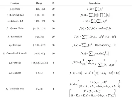
The ten basic benchmark problems summarised in Table 1, can be classified into two groups. The first five functions f1 - f5 are unimodal functions. The unimodal functions here are used to test if MBOA-BIDE can maintain the fast-converging feature compared with the other methods. The next five functions f₆ - f10 are multimodal functions with many local optima. These functions can be used to test the global search ability of the algorithm in avoiding premature convergence.

3.2. The effect of population size N

We set MBOA-BIDE with different population size (N = 10, 40, 50, 100, 150 and 200). The results of differ-ent population size are presdiffer-ented in Table 2. From Table 2, we can see that population size N with 40 is pro-viding the best results in eight of the ten selected functions.

Table 1. Benchmark functions.

Function Range D Formulation

1

f : Sphere [−100, 100] 30

2

f : Schwefel 2.22 [−10, 10] 30

3

f : Schwefel 1.2 [−100, 100] 30

4

f : Quartic Noise [−1.28, 1.28] 30

5

f : Rosenbrock [−30, 30] 30

6

f : Rastrigin [−5.12, 5,12] 30

7

f Generalized Schwefel [−500, 500] 30

8

f : Foxholes [−65.536, 65.536] 2

9

f : Sixhump [−5, 5] 2

10

f : Goldstein price [−2, 2] 2

assigned a rank with a gap (gap is determined based on the number of equally performing algorithms). Table 3

provides the ranks of the different population size and the average rank for all the functions based on mean per-formances. Based on the average ranking, the order of performance obtained is N = 40 followed by N = 50,

N = 10, N = 100, N = 150 and N = 200 respectively.

Figure 1 presents the histograms that indicate the number of times each population size N have achieved the ranks in the range of 1 to 6. It can be seen that N = 40 achieves the top rank as compared to the other dif-ferent population size.

3.3. The effect of magnetic field

B

To study the effects of B in MBOA-BIDE, we use f5, f7 and f8 for testing the performance of MBOA- BIDE. Firstly we suppose B is constant (B = 1, 3, 5, 7, 10), and study the effect of B on test functions. Secondly, we also study the effect of B varying with generation increases as follows:

• B is linearly increases from 1 to10 (B = 1 - 10 LINER).

• B is exponentially increases from 1 to 10 (B = 1 - 10 EXP )

• B is linearly increases from 1 to 100 (B = 1 - 100 LINER)

• B is exponentially increases from 1 to 100 (B = 1 - 100 EXP).

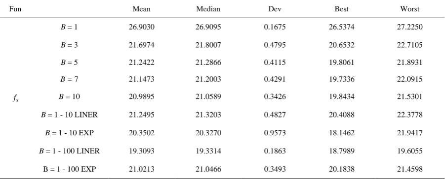
The results are shown in Table 4. From Table 4, for f5, we can see that when B is constant, B = 10, the method can achieve better performance, when B = 1 - 100 LINER can achieve better performance on f₅. For

7

f , when B = 3 and B = 1 - 100 EXP, the method can achieve better performance. For f8, we can see that when B = 1 and B = 1 - 10 LINER can achieve better performance.

Figure 2 Presents the line chart and histograms that indicate the mean, best and median values each B _have

achieved for f7, respectively. From Figure 2, we can see when B = 1 - 100 EXP, MBOA-BIDE achieve the 2

1

( ) in i f x =

∑

1 1

( ) n _i n _i

i i

f x =

∑

∏

2

1 1

( ) ni ( ij j)

f x =

∑ ∑

4 1

( ) n_i i [0,1)

f x =

∑

1 2 2 2

1 1

( ) ni [100( i i) ( i 1) ] f x =

∑

2 1

( ) n [ _i 10 cos(2 _i) 10

i

f x =

∑

1

( ) _in isin( i

f x =

∑

25 ₁ 2 1 1 1 1 ( ) [ ]

500 j _{( )6}

i ij i

f x

j x a

− = = = + + −

∑

_∑

2 4 6 2 4

1 1 1 1 2 2 2

1

( ) 4 2.1 4 4

3

f x = x − x + x +x x − x + x

2 1 2

2 2

1 1 2 1 2 2

2 1 2

2 2

1 1 2 1 2 2

1 ( 1)

( )

(19 14 3 14 6 3 )

30 (2 3 )

18 32 12 48 36 27 )

x x

f x

x x x x x x

x x

x x x x x x

Figure 1. Histogram of individual mean ranks.

Table 2. Statistical results obtained by MBOA-BIDE with different population size N.

Func. N = 10 N = 40 N = 50 N = 100 N = 150 N = 200

1

f

Mean 0 0 0 0 2.5201e−254 4.5896e−181

Dev 0 0 0 0 0 0

Rank 1 1 1 1 5 6

2

f

Mean 0 0 0 4.3137e−209 3.3968e−129 5.5820e−91

Dev 0 0 0 0 6.3405e−129 1.2236e−90

Rank 1 1 1 4 5 6

3

f

Mean 0 0 0 3.0876e−312 5.5975e−182 1.0773e−124

Dev 0 0 0 0 0 3.8100e−124

Rank 1 1 1 4 5 6

4

f

Mean 1.4263e−05 2.2258e−05 1.1082e−05 2.7951e−05 2.2837e−05 2.7755e−05

Dev 1.0928e−05 1.7502e−05 1.1717e−05 2.8866e−05 1.5794e−05 3. 4894e−05

Rank 2 3 1 6 4 5

5

f

Mean 21.4943 21.3003 22.1453 23.6719 24.2513 24.6209

Dev 0.7394 0.4264 0.3933 0.2229 0.2143 0.1610

Rank 2 1 3 4 5 6

6

f

Mean 0 0 0 0 0 0

Dev 0 0 0 0 0 0

Rank 1 1 1 1 1 1

7

f

Mean −1.1199e+04 −1.1808e+04 −1.1535e+04 −1.0843e+04 −1.0664e+04 −1.0807e+04

Dev 1.0496e+03 1.0526e+03 1.5453e+03 1.9108e+03 1.7327e+03 1.5578e+03

Rank 3 1 2 4 6 5

8

f

Mean 7.8914 2.5827 2.4521 1.1949 0.9980 0.9980

Dev 4.0483 3.3070 3.6346 1.0783 4.1884e−12 5.8272e−12

Rank 6 5 4 3 1 1

9

f

Mean −1.03162842 −1.03162845 −1.03162845 −1.03162845 −1.03162845 −1.03162845

Dev 3.2639e−08 6.5144e−10 9.0922e−10 3.3173e−10 4.8852e−10 7.3936e−10

Rank 6 1 1 1 1 1

10

f

Mean 3.0000 3.00000 3.0000 3.00000 3.00000 3.00000

Dev 3.7073e−07 5.7118e−08 3.7689e−08 5.3505e−08 2.3598e−08 3.1246e−08

Rank 1 1 1 1 1 1

0 2 4 6 8

N=10 N=50 N=150

Figure 2. Histogram of statistical results of MBOA-BIDE with different B values

Table 3. Rank table for the mean values.

Fun N = 10 N = 40 N = 50 N = 100 N = 150 N = 200

1

f 1 1 1 1 5 6

2

f 1 1 1 4 5 6

3

f 1 1 1 4 5 6

4

f 2 3 1 6 4 5

5

f 2 1 3 4 5 6

6

f 1 1 1 1 1 1

7

f 3 1 2 4 6 5

8

f 6 5 4 3 1 1

9

f 6 1 1 1 1 1

10

f 1 1 1 1 1 1

Avg. rank 2.4 1.6 1.6 2.9 3.4 3.8

Table 4. Statistical results obtained by MBOA-BIDE with different B values.

Fun Mean Median Dev Best Worst

5

f

B = 1 26.9030 26.9095 0.1675 26.5374 27.2250

B = 3 21.6974 21.8007 0.4795 20.6532 22.7105

B = 5 21.2422 21.2866 0.4115 19.8061 21.8931

B = 7 21.1473 21.2003 0.4291 19.7336 22.0915

B = 10 20.9895 21.0589 0.3426 19.8434 21.5301

B = 1 - 10 LINER 21.2495 21.3203 0.4827 20.4088 22.3778

B = 1 - 10 EXP 20.3502 20.3270 0.9573 18.1462 21.9417

B = 1 - 100 LINER 19.3093 19.3314 0.1863 18.7989 19.6055

B = 1 - 100 EXP 21.0213 21.0466 0.3493 20.1838 21.4598

-1.40E+04 -1.20E+04 -1.00E+04 -8.00E+03 -6.00E+03 -4.00E+03 -2.00E+03 0.00E+00

Mean Best Median

B=1

B=3

B=5

B=7

B=10

B=1-10LINER

B=1-10EXP

B=1-100LINER

Continued

7

f

B = 1 −1.0623e+04 −1.0600e+04 247.5844 −1.1137e+04 −1.0214e+04

B = 3 −1.0880e+04 −1.1211e+04 1.0098e+03 −1.1755e+04 −8.3927e+03

B = 5 −8.4505e+03 −8.3105e+03 1.2271e+03 −1.1428e+04 −6.8399e+03

B = 7 −7.2628e+03 −7.1560e+03 548.8644 −8.4595e+03 −6.3355e+03

B = 10 −7.4822e+03 −7.5949e+03 647.8553 −8.8086e+03 −6.0637e+03

B = 1 - 10 LINER −1.1722e+04 −1.2147e+04 1.3761e+03 −1.2320e+04 −6.9487e+03

B = 1 - 10 EXP −1.1799e+04 −1.1768e+04 134.5198 −1.2219e+04 −1.1609e+04

B = 1 - 100 LINER −9.1931e+03 −9.1373e+03 1.3684e+03 −1.2563e+04 −6.5952e+03

B = 1 – 100 EXP −1.2099e+04 −1.2530e+04 1.3411e+03 −1.2553e+04 −7.2080e+03

8

f

B = 1 3.3981 0.9980 4.1130 0.9980 12.6705

B = 3 5.6198 4.5408 3.8717 0.9980 12.6705

B = 5 7.1337 8.2029 4.7696 0.9980 12.6705

B = 7 5.8563 3.9683 4.4765 0.9980 12.6705

B = 10 6.3849 6.1614 3.6604 0.9980 12.6705

B = 1 - 10 LINER 1.8220 0.9980 2.4891 0.9980 12.6705

B = 1 - 10 EXP 2.8240 0.9980 3.8456 0.9980 12.6705

B = 1 - 100 LINER 2.7863 0.9980 3.8309 0.9980 12.6705

B = 1 - 100 EXP 2.2053 0.9980 3.0987 0.9980 12.6705

performance on f7.

3.4. The Effect of c1 and c2

Firstly we suppose that c1 and c2 is constant, and study the effect of c1 and c2 on three test functions. We set c1 + c2 = 1, and c1 with different values (0.1, 0.3, 0.5, 0.7, 0.9). Secondly, we also study the effect of c1 and c2 varying with generation increases. The parameter settings are as follows:

• c₁ = 0 - 1 L: c1 is linearly increases from 0 to1, c2 = 1 - c1;

• c₂ = 0 - 1 L: c2 is linearly increases from0 to1.c1 = 1 - c2;

• c₁ = 0.1 - 1 E: c1 is exponentially increases from 0.1 to1, c2 = 1 - c1;

• c₂ = 0.1 - 1 E: c2 is exponentially increases from 0.1 to 1, c1 = 1 - c2;

• c₁ = 0 - 2 L: c1 is linearly increases from 0 to2, c2 = 2 - c1;

• c₂ = 0 - 2 L: c2 is linearly increases from0 to2, c1 = 2 - c2; The statistical results are shown in Table 5.

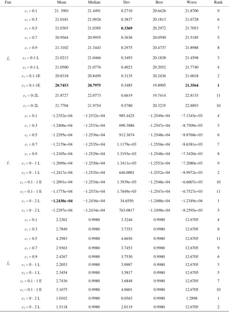
From Table 5 and Table 6, we can see that for f5, c2 = 0.1 - 1 E obtain the best performance. For f7 and 8

f , c1 = 0 - 2 L obtain the best performance. and based on the average ranking, the order of performance ob-tained is c = 0 - 1 L followed by 2 c1 = 0 - 2 L, c1 = 0 - 1 L, c2 = 0 - 2 L, c1 = 0.3, c1 = 0.1, c1 = 0.1 - 1 E, c1 = 0.9, c1 = 0.7, c2 = 0.1-1E and c1 = 0.5, respectively.

4. Conclusion

Table 5. Statistical results obtained by MBOA-BIDE with different C1 and C2 values.

Fun Mean Median Dev Best Worst Rank

5

f

c1 = 0.1 21. 3901 21.4491 0.2710 20.6426 21.8700 9

c1 = 0.3 21.0181 21.0926 0.3837 20.1813 21.6728 6

c1 = 0.5 21.0303 21.0385 0.3369 20.2972 21.7053 7

c1 = 0.7 20.9564 20.9955 0.3636 20.0590 21.5185 5

c1 = 0.9 21.3102 21.3443 0.2975 20.4737 21.8988 8

c1 = 0-1 L 21.0213 21.0466 0.3493 20.1838 21.4598 3

c2 = 0-1 L 21.0500 21.0776 0.4023 20.2052 21.7740 4

c1 = 0.1-1E 20.8318 20.8450 0.3135 20.2436 21.6018 2

c2 = 0.1-1E 20.7453 20.7975 0.3485 19.8905 21.3564 1

c1 = 0-2L 21.8727 22.0773 0.6619 19.7414 22.8133 11

c2 = 0-2L 21.7704 21.9754 0.5780 20.3235 22.8893 10

7 f

c1 = 0.1 −1.2352e+04 −1.2532e+04 985.4425 −1.2549e+04 −7.1345e+03 4

c1 = 0.3 −1.2406e+04 −1.2533e+04 690.3886 −1.2547e+04 −8.7509e+03 3

c1 = 0.5 −1.2295e+04 −1.2536e+04 912.3674 −1.2548e+04 −8.8768e+03 6

c1 = 0.7 −1.2170e+04 −1.2535e+04 1.1179e+03 −1.2556e+04 −8.6381e+03 7

c1 = 0.9 −1.2105e+04 −1.2529e+04 1.3193e+03 −1.2548e+04 −7.3420e+03 8

c1 = 0 - 1 L −1.2099e+04 −1.2530e+04 1.3411e+03 −1.2553e+04 −7.2080e+03 9

c2 = 0 - 1 L −1.2417e+04 −1.2535e+04 646.0001 −1.2552e+04 −8.9972e+03 2

c1 = 0.1 - 1 E −1.2091e+04 −1.2534e+04 1.3939e+03 −1.2548e+04 −6.6607e+03 10

c2 = 0.1 - 1 E −1.1775e+04 −1.2533e+04 1.7649e+03 −1.2547e+04 −6.7527e+03 11

c1 = 0 - 2 L −1.2430e+04 −1.2436e+04 34.6550 −1.2488e+04 −1.2349e+04 1

c2 = 0 - 2 L −1.2297e+04 −1.2434e+04 763.0817 −1.2498e+04 −8.2595e+03 5

8

f

c1 = 0.1 2.2362 0.9980 3.3244 0.9980 12.6705 4

c1 = 0.3 2.7849 0.9980 3.7353 0.9980 12.6705 8

c1 = 0.5 4.2983 0.9980 4.6656 0.9980 12.6705 11

c1 = 0.7 2.9363 0.9980 3.7453 0.9980 12.6705 9

c1 = 0.9 2.4267 0.9980 3.7530 0.9980 12.6705 6

c1 = 0 - 1 L 2.2053 0.9980 3.0987 0.9980 12.6705 3

c2 = 0 - 1 L 2.3454 0.9980 3.5817 0.9980 12.6705 5

c1 = 0.1 - 1 E 2.7436 0.9980 3.6848 0.9980 12.6705 7

c2 = 0.1 - 1 E 3.1675 0.9980 4.0601 0.9980 12.6705 10

c1 = 0 - 2 L 1.0102 0.9980 0.0563 0.9980 1.2898 1

Table 6. Rank table for the mean values.

c1, c2

Individual ranking of benchmark functions Avg. RANK (R)

5

f f7 f8

c1 = 0.1 9 4 4 5.67

c1 = 0.3 6 3 8 5.67

c1 = 0.5 7 6 11 8

c1 = 0.7 5 7 9 7

c1 = 0.9 8 8 6 6.67

c1 = 0 - 1 L 3 9 3 5

c2 = 0 - 1 L 4 2 5 3.67

c1 = 0.1 - 1 E 2 10 7 6.33

c2 = 0.1 - 1 E 1 11 10 7.33

c1 = 0 - 2 L 11 1 1 4.33

c2 = 0 - 2 L 10 5 2 5.67

sensitive to parameters settings on some functions.

Acknowledgements

This work is partially supported by the National Natural Science Foundation of China under Grant No.61075113, the Excellent Youth Foundation of Heilongjiang Province of China under Grant No. JC201212, the Fundamental Research Funds for the Central Universities No. HEUCFX041306.

References

[1] Storn, R. and Price, K. (1997) Differential Evolution—A Simple and Efficient Heuristic for Global Optimization over Continuous Spaces. Journal of Global Optimization, 11, 341-359. http://dx.doi.org/10.1023/A:1008202821328

[2] Kennedy, J. and Eberhart, R. (1995) Particle Swarm Optimization. IEEE International Conference on Neural Networks, Piscataway, NJ, 1942-1948. http://dx.doi.org/10.1109/ICNN.1995.488968

[3] Müeller, S., Marchetto, J., Airaghi, S. and Koumoutsakos, P. (2002) Optimization Based on Bacterial Chemotaxis. IEEE Transactions on Evolutionary Computation, 6, 16-29. http://dx.doi.org/10.1109/4235.985689

[4] Mo, H.W. (2012) Research on Magnetotactic Bacteria Optimization Algorithm. The 5th International Conference on Advanced Computational Intelligence (ICACI 2012), Nanjing, 423-427.

http://dx.doi.org/10.1109/ICACI.2012.6463198

[5] Mo, H.W. and Xu, L.F. (2013) Magnetotactic Bacteria Optimization Algorithm for Multimodal Optimization. IEEE Symposium on Swarm Intelligence (SIS), Singapore, 240-247.

[6] Faivre, D. and Schuler, D. (2008) Magnetotactic Bacteria and Magnetosomes. Chemical Reviews, 108, 4875-4898. http://dx.doi.org/10.1021/cr078258w

[7] Mitchell, J.G. and Kogure, K. (2006) Bacterial Motility: Links to the Environment and a Driving Force for Microbial Physics. FEMS Microbiol. Ecol., 55, 3-16. http://dx.doi.org/10.1111/j.1574-6941.2005.00003.x

[8] Mo, H.W., Liu, L.L., Xu, L.F. and Zhao, Y.Y. (2014) Performance Research on Magnetotactic Bacteria Optimization Algorithm Based on the Best Individual. The 6th International Conference on Bio-inspired Computing (BICTA 2014), Wuhan, 318-322.

[9] Mo, H.W. and Geng, M.J. (2014) Magnetotactic Bacteria Optimization Algorithm Based on Best-r and Scheme. 6th Naturei and Biologically Inspired Computing, Porto Portgal, 59-64.

http://dx.doi.org/10.1109/ICNC.2014.6975877

[11] Mo, H.W., Liu, L.L. and Xu, L.F. (2014) A Power Spectrum Optimization Algorithm Inspired by Magnetotactic Bac-teria. Neural Computing and Applications, 25, 1823-1844. http://dx.doi.org/10.1007/s00521-014-1672-3

[12] Mo, H.W., Liu, L.L. and Geng, M.J. (2014) A New Magnetotactic Bacteria Optimization Algorithm Based on Moment Migration. 2014 International Conference on Swarm Intelligence, Hefei, 103-114.