Dynamic Oligopolistic Pricing with Endogenous Change in Market Structure and Market Potential in an Epidemic Diffusion Model

Dynamic Oligopolistic Pricing with

Endogenous Change in Market Structure

and Market Potential in an Epidemic

Diffusion Model

Ziesemer, Thomas

U Maastricht

1993

Online at

https://mpra.ub.uni-muenchen.de/61831/

Dynamic Oligopolistic Pricing with Endogenous Change in Market Structure and Market Potential in an Epidemic Diffusion

Model

Thomas Ziesemer1, Maastricht University, Department of Economics and MERIT, 1993

1. Introduction

In Dosi et al. (1988) there is a repeated claim that economic models should be imperfectly competitive, dynamic and of the disequilibrium type. At first sight this seems to be demanding too much from one paper. However, in this paper it will be

shown that adding an epidemic diffusion model to a simple static monopoly model and to duopoly models generates all

three properties.

After having mainly been used as an empirical tool without explicit supply considerations, the epidemic diffusion

model has begun a second career as an information technology constraint imposed on monopoly models quite common in

economic theory (see Glaister 1974, Metcalfe 1981, Amable 1992, Stoneman 1983, ch. 9, and Mahajan, Muller and Bass

1990 for an introduction to the literature on "diffusion and supply"). Glaister (1974), starting from an epidemic information

diffusion assumption with an exogenous long-run equilibrium value of demand, derived a non-logistic diffusion curve

skewed to higher growth rates in earlier product phases and continuous intertemporal price differentiation. Since that time

the marketing literature has used it in the framework of dynamic optimization and differential games. Metcalfe (1981)

assumed an epidemic demand curve and derived a sigmoid diffusion curve using a monopoly mark-up assumption on the

supply side and the assumption that diffusion is proportional to profits. Amable (1992) extended this analysis to allow for

increasing returns and competing technologies.

This literature has been developed with the intention of improving the theoretical explanation of the observed

sigmoid diffusion curves. Very often these curves show a logistic or skewed diffusion pattern. Several non-epidemic

approaches to explain these patterns have been tried in the literature. The introduction of learning economies is used in the

models by Bass (see Mahajan, Muller and Bass 1990) and Stoneman and Ireland (1983). However, in the former the

diffusion curve derived depends on the specification of an exogenously imposed shift function, which bears great similarity

with the epidemic functions used in the literature mentioned above, and in the latter on a special relation between price

and threshold adopter derived from the imposition of a distribution of firm size that again bears great similarity with the

types of functions used in epidemic models. Soete and Turner (1984) use the assumption of N techniques in a classical

growth model. At the macro level there is a classical investment function from which sectoral investment deviates

1 I would like to thank Bruno Amable for correspondence, Paul Diederen, Theon van Dijk, René Kemp, Bart

Verspagen and Adriaan van Zon for helpful discussions, Marc van Wegberg and Arjen van Witteloostuijn for their detailed

comments on the conference version, Gene Grossman for providing me with the written version of his conference remarks

and very helpful comments on the second but last version and Reinoud Joosten, Hans Peters and Jerry Silverberg for

positively (negatively) if the sector in question has a higher (lower) rate of profit than the average. Asymptotically, the best-practice technique approaches a 100% share of capital, KN, in total capital, K. KN/K follows a sigmoid diffusion curve.

The way any technique α gains capital from inferior and loses capital to superior techniques bears great formal similarity with the way a product loses demand to a new product and gains from older products in the purely empirical "law of

capture" of Norton and Bass (1992). Vintages of capital with a finite horizon optimization model to investigate intra-firm

diffusion are used in Felmingham (1988). Investments made during the early periods have a correspondingly longer

productive lifetime. The lower the discount rate and the higher the expected prices, the larger investment will be. Therefore

investment is first increasing, then decreasing and the vintage capital stock has a sigmoid form.

The examples given above are on the borderline between evolutionary and (neo)classical economics and the

marketing hybrid of the two. A survey of the microeconomic literature can be found in Reinganum (1989). Silverberg, Dosi

and Orsenigo (1988) broadly introduce the evolutionary literature and Mahajan, Muller and Bass (1990) the marketing

literature. Chatterjee and Eliashberg (1990) connect the marketing literature to the microeconomic literature, thereby

giving the epidemic diffusion model and the marketing literature the status of microfounded aggregates.

This paper uses Amable's version of the model (consisting of a linear estimate of a demand curve, a linear quadratic

cost curve and a logistic diffusion curve) and four types of imperfectly competitive behaviour — monopolistic

intertemporal profit maximization, a dynamic Bertrand oligopoly, and a duopolistic differential game with endogenous

market potential, which leads to a Stackelberg-leadership situation or a phase of pure monopoly.

Neither endogenous market potential nor endogenous change in market structure have been treated in the

differential games literature using the epidemic diffusion model or similar constructs (see Mahajan, Muller and Bass 1990

and Dockner and Jorgensen 1988).

The structure of the paper is as follows. In Section 2 the basic elements of Amable's model are presented.

Intertemporal profit maximization results for the case of a slightly extended version of Jorgensen's (1983) pure monopoly

model are derived in Section 3 to facilitate the understanding of the differential game presented later. Section 4 looks at the

results of an oligopolistic market structure where n firms producing homogeneous goods in an otherwise unchanged

model. In Section 5 it is assumed that consumers associate the product with the name of one of two firms; a differential

game of profit maximizing duopolists leads to either monopoly profits for one of the firms and for the other to first positive,

then zero profits and finally exit, or a Stackelberg leader/follower constellation. The Stackelberg leadership-follower

constellation is analyzed in Section 6. In all cases variants of sigmoid diffusion curves are obtained. In Section 7 the results

2. Basic Elements of the Models

The model consists of a linear-quadratic total cost function in output y:

𝐶 = 𝑐0𝑦 + 𝑐1𝑦2 (1)

(where c₀ 0,c₁or0 indicates whether unit costs are rising or falling) and a possibly correct estimate of potential market demand

𝐷 = 𝑎0 − 𝑎1𝑝, 𝑎0, 𝑎1 > 0 (2)

where D is the long run demand potential for given p. Moreover, the choice of D and y is restricted by the epidemic

(information) diffusion curve:

𝑦̇ ≡𝑑𝑦_𝑑𝑡 = 𝛽𝐷𝑦 (1 −𝑦_𝐷) , 𝛽 > 0 (3)

Eq. (3) mirrors the assumption that consumers get to know or forget the product only slowly, depending on sales already

made or the number of persons who have bought the product, y, multiplied by the probability, 1 - y/D, that they meet

somebody who is part of the market potential and does not know the product. The specification used in eq. (3) is known as

the Chow logistic (see Stoneman 1983, p. 70). Glaister used the model for the analysis of the diffusion of consumer

products, and Metcalfe used it for the analysis of diffusion of production technologies. In both contributions, the quantity

sold and the number of adopters are identical, implying that each individual buys or hires one unit per period, an

assumption also widespread in the marketing literature (see Mahajan, Muller and Bass 1990). In a later section we consider a model with two such information diffusion technologies for one firm as initiated by Amable (1992). y, D and p depend on time t.

The epidemic model considers a purely random process of diffusion of knowledge about the existence of a product or

technology and the desire to buy it. The existence of two classes of individuals, one of which knows and buys the product

and one that does not, is analogous to two classes of people with respect to a disease, one of which is randomly infected

and the other is not. Once the product is known there is no uncertainty with respect to quality or price. The assumption of a

purely random process is of course an exaggeration that emphasizes the costlessness of information diffusion. In the

variants that consider diffusion and supply together, labour investment of household into the search for new products, or

advertisement costs of sellers are neglected (for an introduction to the epidemic diffusion models see Thirtle and Ruttan

1987, ch. 3). Efforts to analyze price policy and advertising together yield untractable differential games if goodwill

dynamics are added. Therefore advertising is not considered here. Instead, the focus will be on price policy and market

structure. Before one proceeds to draw managerial consequences, the above-mentioned simplifications should be taken

into consideration. However, complexity sometimes requires us to treat things separately.

on profits. Amable (1992) assumes that the parameters of the model are constant over time and known to the firm at each

moment but not for the future. We make the same assumption in Section 4, but in Sections 3, 5 and 6 we add the

assumption that the firm knows the constancy of parameters over time.

In the next section we shall investigate the model under the assumption of monopolistic behaviour. This is based

upon S. Jorgensen's (1983) contribution, which serves as a reference model for the later oligopolistic models in this paper.

We do not consider the microfoundation of eqs. (2) and (3) (see Oren and Schwartz 1988 and Chatterjee and Eliashberg

1990 on this point) or the marketing instruments that provide the firm with estimates of them.

The logistic diffusion curve y(t) derived for constant D from eq. (3) is an empirically well-established relation (see

Rosegger 1986, ch. 9 and Coombs, Saviotti and Walsh 1987, ch. 5.6 for descriptive realism, and Mahajan, Muller and Bass

1990 and Karshenas and Stoneman 1992 for econometric estimations and tests of models) and will turn out to be the

result of the monopolistic (Section 3) and oligopolistic (Section 4) considerations and of the change in market structure

(Sections 5 and 6) here. Therefore we try to contribute to the literature on diffusion and supply with special emphasis on

market structure.

3. Intertemporal Profit Maximization with a Single Diffusing Technology

If the monopolist producing y maximizes intertemporal profits for an infinite horizon subject to eq. (3) because no

(potential) competitor is threatening his position, the Hamiltonian for his program is

H = (p-c₀-c₁y)y + λ[βy(a₀-a₁p )-βy2_].

The first order conditions for a singular solution are eqs. (4), (5) and lim t  e -ρtλ

(t) = 0:

δHδp = y+λβy(-a₁) = 0. (4)

The economic problem here is that high prices increase temporary profits but decrease future profits by reducing the speed

of diffusion. As the Hamiltonian is linear in p a singular solution is optimal for some time phase if it exists. During such a phase a singular solution requires a constant λ, following from eq. (4):

The shadow price of y is the inverse of the impact of p on the growth rate of y, βa1. The first order condition for y is (with

discount rate ρ)

From the solution for λ and its constancy we obtain

λ = 1(βa₁).

               

 _{/ 2 [ ( ) 2 ]} 

1 0 1

0 c y a a p y

c p Y

-p+c₀ + c₁2y - (βa₁)-1_[β_(a

0 - a1p) - 2βy] = -ρ(βa1)

-1_{. (5’)}

The condition from static theory that marginal revenue should equal marginal cost is modified by two dynamic terms here, one due to diffusion and one due to discounting. Terms containing p are identical up to their sign and thus can be dropped. Then solving for y yields:

y* _{= ( -}ρβ

-c₀a₁+a₀)[2(c₁a₁+1)]. (6)

y* is a constant value here. This solution differs from the solution of the static monopoly model only by the term ρ/β. The monopoly solution eq. (6) with diffusion is lower than the static monopoly solution because of the impatience expressed

by the positive discount rate. Here is the change of y is zero and the price is determined by a0 - a1p *

= y*. As a consequence in this phase the last term subtracted on the left hand side of eq. (5') is negative. If ρ is close to zero, price then has to be

higher than marginal cost. This is all the more the case if ρ»0. For profits to be positive for all ρ we must have a0 - c0a1 > 0.

For a static monopoly solution to exist (ρ  0) and y* to be positive for small ρ, eq. (6) requires that c1a1 + 1 > 0, which we

shall assume henceforth unless noted otherwise.

However, for y(0) < y* (where y(0) may be the sales to workers producing the product who are the most natural

candidates to know first about the existence of the product) there must be a phase where this value is approached. This

requires that the change of y is zero and therefore some p'  p* is sufficient to reach the singular solution. However,

Jorgensen (1983) shows that for c1 = 0 a most rapid approach to a singular solution reached by prices as low as possible is

the optimal solution. These are introductory prices to be defined below. During such a phase y is lower than D and supply is therefore lower than estimated potential demand. In this sense there is a temporary disequilibrium due to slow diffusion. Of course, "one can turn any disequilibrium model into an equilibrium equivalent [if an equilibrium exists, T.Z.] and vice versa by a suitable definition of the information sets and perceptions of adopting agents" (Metcalfe 1988, p. 561).

Due to the linearity of H in p a lower bound for p, p', has to be imposed at which the diffusion of knowledge takes place. Some examples of such bounds can be discussed for the purpose of illustration. If the chosen p' goes to minus infinity one

obtains jumps (impulse control) in the stock variable y. As this is at variance with the idea of slow diffusion we do not

consider this possibility. Free sample copies, hence p' = 0, are a possibility as well. However, the accompanying losses

during a phase with prices lower than costs require credit that can be repaid only in the singular solution phase with

positive profits, and therefore is an unnecessary complication. p' = max (c0, c0 + c1y*) ensures non-negative profits in the

introduction phase. Even p' = p* would be a candidate because y* would be approached from any value y(0) < y*. For any such value we have a diffusion process that stops increasing at y*. For a graphical summary of the solution see Figures 1 and 2. During the introductory phase with the lower price price p', the firm moves along the (higher) diffusion curve going

through D'. Once y* = D* is reached this curve is no longer relevant because the change of y becomes zero as the price

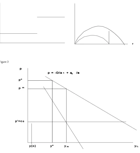
jumps to the higher p*. In spite of a jump of the price there is no corresponding jump in the quantity because the new price implies constant y. The product is no longer made better known because one prefers to have high profits now, if ρ > 0. The equilibrium value y* = D* belongs to a diffusion curve that has not been followed, because there was a jump from D'(p') to D*(p*). As ρ approaches zero the solution approaches that of the static Cournot monopoly. The comparison with Cournot monopoly is illustrated in Figure 3 below for Jorgensen's case with c1 = 0 and p' = c0, where MR is marginal revenue, and ym,

pm is the static monopoly solution. Starting from y(0), y grows at p' = c0 until y *

Figure 1: p on the vertical, t on the horizontal axis Figure 2: dy/dt on the vertical axis

Recall that Glaister (1974) regarded two prices as the more realistic case compared to the permanent intertemporal

price differentiation obtained in his model. The linearity of the Hamiltonian which generates this solution with two prices is

due to the insertion of a linear demand function (see Feichtinger 1982, p. 240) into the Chow logistic, which is the simplest

special case of the Bass model, which in turn is the preferred one of several possible variants (see Stoneman 1983) in the

marketing literature and generates a variant of discontinuous price policy in models of diffusion and supply. If one gives up

one of these specifications the price paths will be either that

penetration in the marketing literature) or

ii) of Robinson and Lakhani (1975) for optimizing and Metcalfe (1981) for non-optimizing behaviour under supply

constraints, both with continuous price differentiation from high to low prices (market skimming).

In Metcalfe's case diffusion may depend strongly on making profits, which requires high introductory prices, whereas

in the Robinson and Lakhani case the fall in prices is due to falling costs and positive discount rates. The cases of

continuously falling or increasing prices as well as a combination of both were contained in Spremann (1975). The

specifications for the case of discontinuous price policy emphasized here will turn out below to be a starting point for

tractable differential games because these are the simplest possible of all specifications used in the literature.

4. Price Policy in a Dynamic Bertrand Duopoly

In this section we use the same model as above but assume that there are n firms introducing the new product at the same

time. Patenting is excluded. Knowledge about the existence of the product again works as in eq. (3). However, the oligopolists now compete for the buyers, y, who know of the product:

The upper indices of the supply terms on the right-hand side of the equation are the indices of the firms. Buyers are

assumed to be perfectly informed about the prices of all firms such that eq. (2) holds with p = min [p1, p2, ... , pn]. We assume that all firms have identical cost functions. As outputs yi and prices pi are fast variables, given the value of the slow variable y, the model is symmetric with respect to the firms and therefore they are assumed to produce the same quantities

yi = y/n. These assumptions are used in the following differential game:

𝑀𝑎𝑥𝑝𝑖𝑝𝑖𝑦𝑖 − (𝑐0+ 𝑐1𝑦𝑖)𝑦𝑖

s.t. (2), (3) and 𝑦_𝑖 =𝑦_𝑛, 𝑝_𝑖 ∈ [𝑐₀+ 𝑐₁𝑦_𝑖,𝑎_𝑎1

0 ]

with c0 + c1yi as a lower bound for pi as in section 3. For n=1 this game yields the same results as section 3. For n>1 the

rationing rule is yi = y/n, all firms choose identical quantities and prices because they are identical in all respects. Instead of

(5') and (6) one gets for a singular solution:

𝑝𝑖(1 −_{𝑛) = 𝑐}1 0+ 2𝑐1𝑦_{𝑛 −𝑛𝑎1}𝑎0 +_{𝑛𝛽𝑎1}𝜌 +_{𝑛𝛽𝑎1}2𝛽𝑦

which is identical to (5') for n=1, and

𝑦∗ 𝑛 =

𝑎0−𝑎1−𝜌_𝛽

𝑛−1+2(𝑎1𝑐1+1) (7)

which is identical to (6) for n=1. In (6) p dropped out because n=1. Therefore a solution for y was obtained which had to be approached gradually in a transition to the singular solution. For n>1, p does not drop out now. Given the initial value for y/n, p is determined in the equation that is similar to (5') and the shadow price can be determined such that a singular solution is valid from the beginning. No transition is necessary. Insertion of the price equation into the differential equation

for y would allow to analyse the dynamics of y again. Under the assumption that the numerator and the denominator of the

stationary solution of y are both positive one gets the same type of a curve as in Figure 2. In this model profits will in general

be positive as in the model of section 3.

A rather similar model is that of Rao and Bass (1985), where products are also homogeneous and therefore prices

have also to be identical across firms, but costs are dependent on cumulative output. The model by Eliashberg and Jeuland

(1986) differs from that of Rao and Bass (1985) in that they consider differentiated products with homogeneous products

as the special case of a huge impact of price differences and no learning effects in the cost functions. For that limiting case

their (very complex) model is one with an exogenous market potential.

In summary, the introduction of competitors has made a continuous price policy out of what was a discontinuous

price policy in the previous, monopolistic model.

5. A Duopolistic Differential Game with Endogenous Market Potential and Transition to Monopoly or Stackelberg

Leadership

own reputations. The products of the two firms considered are imperfect substitutes. The difference between the products

is indicated by the name or reputation of the firms producing with identical unit cost functions

c = c₀+c₁y.

Consumers knowing about the product of a firm infect those consumers who do not know either of the two

firms or their product. The epidemic process is then (see Amable 1992)

𝑦̇1 = 𝛽𝑦𝑖(𝐷 − 𝑦𝑖− 𝑦𝑗) i = 1, 2; j≠i

These are two diffusion processes — one for each firm's reputation or number of clients — with the same growth rates.

This dynamic process imposes identical growth rates on the reputations of the two firms, which is a rather strong dynamic

rigidity. However, it simplifies the analysis considerably because the difference in levels of the yi will be determined by their

initial values and the common growth rate (on the tractability of differential games with respect to the problem at hand see Dockner and Jorgensen 1988). In the y1-y2-plane the duopoly then moves along a ray through the origin determined by the

initial values. If a differential equation drives yi upwards (downwards) then the firm's quantity cannot grow faster (decline

slower) and by assumption it can never jump. The firm can sell less but not more than indicated by the differential

equation.

Overall potential demand D is assumed to be

D = a₀-a₁p₁2-a₁p₂2.

This demand function can be derived as a special case of the demand functions for imperfect substitutes:

D1 = e1-b1p1+d1p2, D2 = e2+b2p1-d2p2

Summing left and right hand sides yields

Assuming b1 - b2 = d2 - d1 and defining e1 + e2 a0 and b1 - b2 = d2 - d1 a1/2, the above demand function is obtained. a1/2

is positive if own-price effects are stronger then cross-price effects. For the case p1 = p2 this demand function reduces to the

demand function in the monopolistic part of the paper. The assumption b1 - b2 = d2 - d1 a1/2 is a strong simplification

which helps to focus on differences in the initial values of market shares as the main point of interest concerning

differences between firms. Which firm becomes known to the buyer is again determined solely by the epidemic random

process operating on a common market potential D for both firms. Both prices have an impact on the speed of diffusion of the knowledge about the existence of the product. High prices increase current profits given a vertical short-run demand

curve yi because yi is a slow variable, and low prices contribute to the diffusion. Therefore individual firms' intertemporal

profit maximization subject to the differential equations takes the form of a duopolistic differential game where each firm

bases its own decision on expectations about the other firm's behaviour concerning price and quantity:

𝑀𝑎𝑥𝑝_𝑖,𝑡1∫[𝑝𝑖 𝑡1

0

𝑦𝑖 − (𝑐0+ 𝑐1𝑦𝑖)]𝑒−𝜌𝑡_{𝑑𝑡, 𝑖 = 1,2}

s.t.

𝑦̇1 = 𝛽𝑦𝑖(𝐷 − 𝑦𝑖− 𝑦𝑗), 𝑖 = 1, 2; 𝑗 ≠ 𝑖,

and y1(0)=y10, y2(0)=y20, t1≥0.

Up until now in the literature such games have only been considered for constant values of D, although endogenous D is held to be desirable (see Dockner and Jorgensen 1988). In that literature prices p1,2 are introduced in a manner that is more

reminiscent of Glaister's β(p) function. We consider the Nash equilibrium for open-loop strategies. Whereas the marketing literature focuses on price policy and profits, we also look at diffusion and change in market structure in connection with

leadership in terms of market shares.

Insertion of D into the differential equation yields the generalized Hamiltonian for firm 1:

The first order conditions for a singular solution phase are the differential equations (3'), λ1(t1) = μ1(t1) = 0, H(t1) = 0,

implying zero profits if finite t1 exists, and

δH₁δp₁ = y₁+λ₁βy₁(-a₁2)+μ₁βy₂(-a₁2) = 0

(where ρ is the discount rate as in the monopolistic model) and

From these first order conditions one can solve for p1 and p2. The results are:

-c₀- (2c₁+ 4a₁)y₁-ρ2(a₁β)+(2a₁)a₀- 4y₂a₁ = p₂

D = a₀-a₁p₁2-a₁p₂2

H₁ = p₁y₁- (c₀+c₁y₁)y₁+λ

1βy1(a0-a1p12-a1p22 -y1-y2), ,+μ1βy2(a0+a1p12-a1p22-y2-y1).

-δ_H

1δy1,=-[p1-c0-2c1y1+λ1β(a0-a1p12-a1p22 -y2- 2y1)-μ1βy2],=λ1-ρλ1

-c₀- (2c₁+ 4a₁)y₂+(2a₁)a₀- 4y₁a₁-ρ2(a₁β) = p₁.

In eqs. (11'') and (12'') y1 and y2 are slow state variables. Therefore they determine those (expected) values of prices which

can be equilibrium prices of a singular solution. From the monopoly model one might have expected that there would

again be a transitionary phase where imposition of values for p1,2 would lead to such a singular solution. However, there is

no reason not to be in a singular solution from the beginning because the equations for a singular solution do not yield results such as y* in the monopoly model that must be approached slowly. The most rapid approach in this case is to begin with (correctly expected) prices as determined by eqs. (11'') and (12''). Insertion of D and the solutions for p1,2 into the

differential equations using y1 + y2 = y yields after some manipulations

Eq. (13) summarizes the development of the market quantity y. y1 and y2 differ only by their initial values and have growth

rates identical to that of y. eq. (13) is graphed in Figure 5. It has an unstable threshold value at

y* _{= (a}

0-a1c0- 2ρβ)(3+a1c1).

Again we assume that the discount rate is sufficiently low to ensure a positive solution y* with positive numerator and denominator. As a consequence of eq. (14) one can draw a no-growth line y1 = - y2 + y* in the y1 - y2-plane (see Figures 6-8).

If the game starts below that line both quantities will be decreasing, and if it starts above it both quantities will be increasing

until a zero profit line is reached. To be able to derive the zero-profit line and to understand the movement to that line we

have to consider the price equations again. Price equations can be rewritten as functions of y and the initial values of y and y1,2 in the following form:

p₂ = -c₀-ρ2(a₁β)+(2a₁)a₀-y[(2c₁+4a₁)y₁₀y₀+4y₂₀(y₀a₁)]

p₁ = -c₀+ (2a₁)a₀-ρ2(a₁β)-y[4y₁₀(y₀a₁)+(2c₁+ 4a₁)y₂₀y₀].

Figure 5 Figure 6

Figure 7 Figure 8

Prices are negatively related to the quantity y. If the initial values were below the threshold value both firms could become smaller and smaller at positive profits with no finite value of t1 existing, because — as will be shown below — zero-profits

lines will be to the right of the no-growth line. Firms would converge to atomistically small suppliers. To understand the

movement to the zero-profit line it is be important to recognize that in spite of the assumption that in the static demand curves a firm's own price has a stronger impact than the other firm's price, b1 - b2 = d2 - d1 = a1/2 > 0, eqs. (11'') and (12'')

imply that a price is more (less) strongly affected by the other firms' quantity than by its own quantity if :

Inserting the price equations into the zero-profit condition pi - c0 - c1yi = 0 yields the zero-profit lines

To illustrate three possible outcomes we distinguish three cases.

Case 1. For c1 = 0 (see Figure 6) the no-growth line has intercepts

y*

= (a₀-a₁c₀- 2ρβ)3

and the zero-profit lines (indicated as ii in Figure 6) becomes

y_i = -y_j+ (a₀-a₁c₀-ρβ)2.

Obviously, zero-growth lines are identical for both firms in this case, have the same slope as the zero-growth line and their intercepts are larger than y*, the intercept of the no-growth line. On whichever ray the firms move to the zero-profit line, they both reach it at the same time t1. From that point in time onwards they may have a weak preference to stay in the

market, which leads to the same results as the Bertrand model of the previous section. Alternatively one or both exit.

Case 2. For c1 > 0 we find that

y* _{= (a}

Therefore horizontal intercepts are clearly ranked and 11, the zero-profit line of firm 1 is steeper than 22, the zero-profit

line of firm 2 (see Figure 7). As the zero-profit lines intersect at the 45 degree line, firm 1 will reach its zero profit line first if

firm 2 has the higher initial value, and the firms therefore move along a ray that is flatter than the 45 degree line. The reason

is that for c1 > 0 the negative effects of one firm's quantity on the other firm's prices indicated in eq. (15) are stronger than

the negative effects of quantities on a firm's own price. When reaching the zero-profit line firm 1 may either exit and leave a

monopoly position for firm 2 or it may weakly prefer a zero profit strategy leaving a Stackelberg leadership position to firm

2, which we analyze below.

Case 3. For c1 < 0 for small c₁ one can show that

y* _{< y} 2_π

2=0,y1=0

< y₂

π1=0,y1=0

and 11 is now flatter than 22, as shown in Figure 8. As a consequence, for y20 > y10 firm 2 will come first to its zero-profit

line because its quantity is depressing its own price more than that of firm 1. Therefore it is either optimal to exit in spite of

having the larger market share or to weakly prefer a zero profit strategy, thus leaving a Stackelberg leader position to firm 1.

Other possible cases might exist because zero-profit lines may be below the no-growth line for c1 « 0. Initial values

above the zero-profit line but below the no-growth line lead to negative growth rates driving the process to the origin.

There will be a phase with negative profits followed by one with positive profits. The question then is whether overall

profits are positive. If a process begins above both lines it will not be started at all because profits become increasingly more

negative. If the zero-profit line lies above the no-growth line an alternative to the singular solution phase might be that firms price at the corner p1 = e1/d1, p2 = e2/d2. Then they move back to the no-growth line with maximum speed. Arriving

there they could price at the no-growth maximum profit price of the singular solution, which may yield higher discounted

long-run profits. However, then the firms no longer are confronted with a diffusion problem.

6. The Stackelberg Leadership Phase

Suppose that firm 2 has gained a Stackelberg Leadership position either because c1 > 0 has brought firm 1 to its

zero-profit line because y20 > y10 or c1 < 0 has brought firm 1 to its zero-profit line because y20 < y10 and it weakly prefers to

stay in the market. Firm 1 may then try to produce y1(t1), the quantity reached during the phase of the duopolistic game,

provided that the differential equation does not produce negative growth rates such that consumers forget the firm. This

will turn out to be no problem, because it will be shown that firm 2 goes to a higher quantity.

The problem for firm 2 from t1 onwards then is

𝑀𝑎𝑥𝑝₂ ∫[𝑝2𝑦2− (𝑐0+ 𝑐1 ∞

𝑡1

𝑦2)𝑦2]𝑑𝑡

s.t. 𝑦̇2 = 𝛽𝑦2[𝑎0−𝑎1(𝑐0+𝑐1𝑦1𝑡1)

2 −

𝑎1𝑝2

2 − 𝑦2− 𝑦1𝑡1)]

given t1 and y1,2(t1) from the previous phase. The current value Hamiltonian can be written as

H = p₂y₂ - (c_o + c₁y₂)y₂ + λ

2y2β [a0 - a1p2  2 - a1 (c0 + c1y1t

1 )  2 - y_1t

First-order conditions for a singular solution phase are: the differential equation, limt e -ρt

= 0 and

and

From these first order conditions one can derive the level of the market quantity y:

𝑦2 = 𝑎0−𝑎1𝑐0−𝜌/𝛽

2(𝑎1𝑐1₂ +1) − 𝑦_1𝑡1

2 (18)

The first term is the value of y2 at the end of the zero-profit line of firm 1 (of the differential game phase), i.e. for π1 = 0 and

y1 = 0 in the y1-y2-plane (see Figure 9). In that plane eq. (18) describes a straight line with slope minus 2 throughy2

π1=0,y1=0 .

Therefore it is steeper than all zero-profit lines of the differential game phase. Since y_1t

1

is a constant and the line

determined by eq. (18) lies to the right of the zero-profit lines of the previous phase, firm 2 moves from the zero profit line

of firm 1 parallel to the horizontal axis to the line of eq. (18), thus extending its market share in the Stackelberg phase

because firm 1 sells less than it's market reputation would allow it to, because it has changed its strategy in order to avoid

running into negative profits, whereas the behaviour of firm 2 must have made both products better known during the

transition to eq. (18), to which we turn now.

Figure 9 Figure 10

For a transition to this singular solution phase of the monopoly for the whole market one would have to define lower

and upper bounds for prices of firm 2 again. Here we assume that the lower bound is the zero-profit condition. However,

when the price jumps down at t1 from its positive profit level for one of the oligopolists (firm 2 in our example) there must

be a jump in dy  d(t₁). The curve of Figure 5 stops at y(t1). From that time onwards the curve of Figure 2 is valid. Its

value of dydt(t+,

1) - where t1 +

is the first moment of the Stackelberg phase - must be higher than the value dydt(t₁)

δHδp₂ = y₂+λ₂βy₂(-a₁2) = 0 (16’)

-δHδy₂ = -{p₂-c₀-c₁2y₂+λ₂β[a_o-a₁p₂2-a₁(c₀+csub1y_1t 1

)2 -y_1t 1

of the differential game phase. There will be a jump to a different diffusion curve when p2 is raised such that the growth

stops at a value of D belonging to the monopoly price. The complete diffusion curve of the whole game is drawn in Figure 10. A similar curve could be derived for the case that firm 1 exits and firm 2 has a monopoly position instead of one of a

Stackelberg leadership.

Whereas in Fershtman, Mahajan and Muller (1990) pioneering advantage is defined with respect to market shares of

a pioneer and a competitor that turn out to be equal in the long run in their model, here market shares are constant during

the differential game phase due to the dynamic rigidity. Pioneering advantage leads to exit or weak preference for staying in with zero profits of the leader if c1 < 0, allowing for Stackelberg-leadership or monopoly profits in a later phase for the one

who was lagging behind in terms of market share in the beginning. Only in the case of an increasing unit cost curve will the

market share "advantage" of the leader not be lost, because in the equations for prices (i.e., eqs. (11'') and (12'') and in

contrast to the properties of the demand functions D1 and D2) cross effects of quantities on competitors prices are larger in

that case than those on a firm's own prices. If unit cost curves are falling the quantities of a firm have a higher influence on

its own price. Then higher initial quantities (pioneer advantage) lead the pioneer to his zero-profit line,

Stackelberg-followership or exit (optimal timing of withdrawing a product from the market). The Stackelberg leader then

extends his market share. This phase is initiated by a downward jump of the price. Another example of a downward jump

of the price can be found in Eliashberg and Jeuland (1986), where a monopolist decreases his price at the moment of entry

of a competitor.

7. Conclusions

In this paper the model used by Metcalfe, Batten and Amable and in the marketing literature has been used to derive the

dynamics of output and price under different behavioral assumptions than in their papers. It seems to me that the

imposition of the epidemic diffusion assumption as a technological constraint on information flows is an interesting

approach to dynamic imperfectly competitive disequilibrium behaviour, although I would not go as far as Batten (1987),

who views this model as competing with the neoclassical growth model. The latter is a general equilibrium model whereas

the Metcalfe and marketing models are partial (dis)equilibrium models. In the following we summarize the results obtained

with this approach.

This paper has started from Jorgensen's (1983) version of the monopoly model. In that version there is an optimal

introductory price and a jump to a long run price that is higher than that of a static monopoly solution under a positive

discount rate. This result differs from the permanent, continuous price differentiation obtained by Glaister (1974), Metcalfe

(1981) and others; disequilibrium growth is found in the introduction phase of the product but not in the phase of a

singular solution.

Allowing for competition one has to make an assumption on whether or not the dynamics of the product becoming

known is associated with the name of the firm. If it is not, firms compete under perfect information for the number of

consumers knowing the product. Under mutually perfect information a zero-profit strategy is the only equilibrium strategy

because for higher prices a competitor can always take over the whole market. As a consequence the two-prices strategy of

the monopoly version of the model is replaced by a continuous price strategy. Before the diffusion process has proceeded

sufficiently the firm will not be on the estimated and possibly true demand curve, and therefore the economy will be in

If the product becomes known and the consumers associate the name of the firm with the product and do not know of

the other firm's supply, then substitutes are imperfect. In a differential game with dynamic rigidity higher prices lead to

higher instantaneous profits but slow down the diffusion. If the initial values are below a critical minimum level the

quantities of both firms will decline towards zero and prices will rise. If the initial values are above a critical minimum level

the quantities will grow and prices will decline. Under decreasing (increasing) cost curves the leader (follower) arrives at his

zero-profit line when the other firm still makes positive profits. If it switches to a zero profit strategy the other firm becomes

Stackelberg leader, and if it exits the other firm gets a monopoly position.

In the latter case we are back in the slightly extended Jorgensen model. In short, epidemic diffusion dynamics

combined with a demand and a cost function can be used in models that are imperfectly competitive, and can also be used

to justify dynamic monopolistic (dis)equilibrium or Stackelberg leadership, both possibly resulting from a duopolistic

differential game.

An alternative version that we shall investigate in a further paper will use individual market potentials Di = ai - bi pi + bj

pj, with bi,j > 0 and individual diffusion curves y_i = βy_i(D_i - y_i). In that case the dynamic rigidity will vanish and there

will be competition for market potential. The main problem will presumably be the tractability of the differential game.

Advertising may be added to the model by making β dependent on the expenditures for advertising. This would avoid

adding additional differential equations for goodwill.

The purely empirical literature as far as it is based on the epidemic model considers the sigmoid or similar diffusion

patterns which can be generated formally by the models mentioned above. In the models, however, diffusion is driven by

firms' price policy, investment or output decisions. The models using price policy exhibit a great variety of possible policies.

They are all based on continuous intertemporal price differentiation. To get a better impression of how all of this works it is

necessary to enlarge empirical research to include the price policy and changes in market structure accompanying the

diffusion process. A crucial empirical question will be how the price paths are correlated with the diffusion paths and

perhaps those of other variables.

This paper has looked with somewhat neoclassical eyes at the literature connecting the epidemic diffusion model with

dynamic firm behaviour and therefore ended up in marketing science, where this model is most prominent. It is clear that

evolutionary economists will find this effort to be too neoclassical and will doubt the availability of the necessary

information, and that neoclassical economists will shift emphasis to even better information emphasizing advertising and

search costs of customers. However, I share the marketing literature's view that all of these measures may improve information but will not change the character of the basic problem because advertising and search costs will increase β and will therefore increase the term in our model, but will not necessarily change results radically. However, the models might

become more complicated. We hope that there are more economists outside the marketing field who like parts of all the

three directions of research and are convinced that the epidemic diffusion model has something to offer to neoclassical

economics and deserves the effort of extension to general equilibrium modelling which might make clear what are the

References

Amable, B. (1992), "Competition among Techniques in the Presence of Increasing Returns to Scale", Journal of Evolutionary Economics, 2, 147-158.

Batten, D. (1987), "The Balanced Path of Economic Development: a Fable for Growth Merchants", in Batten, D., J. Casti and

B. Johansson (eds.), Economic Evolution and Economic Adjustment, Heidelberg: Springer-Verlag.

Chatterjee, R. and Eliashberg, J. (1990), "The Innovation Diffusion Process in a Heterogeneous Population: A Micromodelling Approach", Management Science, 36, 1057-1079.

Coombs, R., Saviotti, P. and Walsh, V. (1987), Economics and Technical Change, London: MacMillan.

Dockner, E. and Jorgensen, S. (1988), "Optimal Pricing Strategies for New Products in Dynamic Oligopolies", Marketing

Science, 7, 315-334.

Dosi, G., Freeman, C., Nelson, R.R., Silverberg, G. and Soete, L. (1988), Technical Change and Economic Theory, London:

Pinter.

Eliashberg, J. and Jeuland, A.P. (1986), "The Impact of Competitive Entry in a Developing Market upon Dynamic pricing Strategies", Marketing Science, 5, 20-36.

Feichtinger, G. (1982), "Optimal Pricing in a Diffusion Model with Concave Price-Dependent Market Potential", Operations Research Letters, 1, 236-240.

Felmingham, B.S. (1988), "Intra-firm Diffusion and the Wage Bargain", Economics Letters, 26, 89-93.

Fershtman, C., Mahajan, V. and Muller, E. (1990), "Market Share Pioneering Advantage: A Theoretical Approach",

Management Science, 36, 900-918.

Glaister, S. (1974), "Advertising Policy and Returns to Scale in Markets where Information is passed between Individuals", Economica, 41, 139-156.

Jorgensen, S. (1983), "Optimal Control of a Diffusion Model of New Product Acceptance with Price-Dependent Total Market Potential", Optimal Control Applications & Methods, 4, 269-276.

Karshenas, M. and Stoneman, P. (1992), "A Flexible Model of Technology Diffusion Incorporating Economic Factors with

an Application to the Spread of Colour Television Ownership in the UK", Journal of Forecasting, 11, 577-601. Mahajan, V., Muller, E. and Bass, F.M. (1990), "New Product Diffusion Models in Marketing: A Review and Directions for

Research", Journal of Marketing, 54, 1-26. Reprinted in N. Nakicenovic and A. Grübler (eds.) (1991), Diffusion of Technologies and Social Behaviour, Heidelberg: Springer-Verlag.

Metcalfe, J.S. (1981), "Impulse and Diffusion in the Study of Technical Change", Futures, 13, 347-359.

Metcalfe, J.S. (1988), "The Diffusion of Innovations: an Interpretative Survey", in Dosi, G., Freeman, C., Nelson, R.R.,

Silverberg, G. and L. Soete (eds.), Technical Change and Economic Theory, London: Pinter.

Norton, J.A. and Bass, F.M. (1992), "Evolution of Technological Generations: The Law of Capture", Sloan Management

Review, 66-77.

Oren, S.S. and Schwartz, R.G. (1988), "Diffusion of New Products in Risk-sensitive Markets", Journal of Forecasting, 7,

273-287.

Rao, C.R. and Bass, F.M. (1985), "Competition, Strategy, and Price Dynamics: A Theoretical and Empirical Investigation", Journal of Marketing Research, XXII, 283-96.

Reinganum, J.F. (1989), "The Timing of Innovation: Research, Development, and Diffusion", in R. Schmalensee and R.D.

Robinson, B. and Lakhani, C. (1975), "Dynamic Price Models for New-Product Planning", Management Science, 21,

1113-1122.

Rosegger, G. (1986), The Economics of Production and Innovation, London: Pergamon Press.

Silverberg, G., Dosi, G. and Orsenigo, L. (1988), "Innovation, Diversity and Diffusion: A Self-Organisation Model", The

Economic Journal, 98, 1032-1054.

Soete, L. and Turner, R. (1984), "Technology Diffusion and the Rate of Technical Change", The Economic Journal, 94,

612-23.

Spremann, K. (1975), "Optimale Preispolitik bei dynamischen deterministischen Absatzmodellen", Zeitschrift für Nationalökonomie, 35, 63-76.

Stoneman, P. (1983), The Economic Analysis of Technical Change, Oxford: Oxford University Press.

Stoneman, P. and Ireland, N.J. (1983), "The Role of Supply Factors in the Diffusion of New Process Technology", The

Economic Journal, 66-78.