Comprehensive Study on Computational Methods
for K-Shortest Paths Problem
Kalyan Mohanta
B. P. Poddar Institute of Management & Technology
Kolkata, India
ABSTRACT
The application domains like network connection routing, highway and power line engineering, robot motion planning and other optimization problems require the computation of shortest path. Computations of K-shortest paths provide more (K-1) numbers of backup shortest paths for consideration, which enable the applicability of additional constraints on the particular domains. For instance, a biologist can determine the best of an alignment from the available instances of biological sequence alignments generated from more than one shortest paths computation. The purpose of this paper is to provide a comprehensive review of existing algorithms available for K-shortest paths computation. It will be useful for researcher to implement the effective K-shortest paths computation based on their matching computational requirements over the domain of their interest.
General Terms
AlgorithmsKeywords
Shortest path, K-shortest paths, Optimality principle, Algorithm, Computational complexity
1.
INTRODUCTION
Finding the K-shortest paths in a network (without negative loop) is a classical problem to compute not only the shortest path from the origin to sink, but also determine more (K-1) shortest paths for K > 1. The algorithms available to solve the problem can be classifiable into two categories based on the type of computable path: (a) Algorithms to compute K-shortest paths without any loop, and (b) Algorithms to compute K-shortest paths that may have loops.
Bock, Kantner, and Haynes [1], Pollack [2], Clarke, Krikorian, and Rausan [3], Sakarovitch [4], Azevedo at. al. [5,6,7], Dreyfus [8], Eppstein [9], Shier [10,11,12], Yen [13], Martin at. al. [14] and others propose K-shortest path algorithms without any loop. Hoffman and Pavely [15], Bellman and Kalaba [16], Sakarovitch [4], Martins al. al. [17,18] and others propose algorithms to compute K-shortest paths that may have loops.
This review is carried out to explore the basic types of the algorithms available for computing loop less K-shortest paths between a pair of nodes in a network and to reflect their computational procedure and computational complexity. It also explains the computational advantages over simple version of some algorithms by using techniques of path representations like “implicit path” [9], “sorted forward star form” [19] and others.
The notations and definitions used throughout this review are shown in Section 2. Section 3 explains the representation of paths in K-shortest paths algorithms. Review of the available
K-shortest path algorithms from the computational viewpoints are explained in section 4. A comparison on computational complexity of available K-shortest paths algorithms is given in section 6. Some applications of K-shortest paths algorithm are explained in section 7.
2.
PRELIMINARIES
Let G = N, A denotes an input network with n nodes and m edges, where N = v1, v2, … , vn the finite set of n nodes, and
A = e1, e2, … , em is the finite set of m edges. With no loss of generality, let G is a directed network and every edge ek is an ordered pair i, j of nodes from the network.
Lat a path from source i to destination j is denoted byPij. The K-shortest paths from some source to destination are represented with the nonempty set π = {π1, π2, … , πK} of K-paths in order.
Let the cost of any edge denoted by c ek , is a real number associated with the edgeek and let the cost of any path p is defined as c p = (i,j)ϵpcij.
3.
REPRESENTATION OF PATHS
Computing K-shortest paths from a network requires nodes to store more than one path information in the form of path cost from the source. Particularly the source and the destination node should store K-path information. Information’s may store in the label of each node with the K-tuple of storage. For example πijk may be used to store K different paths from node i to node j for k=1, 2, … , K.
Due to the unavailability of any a-prior information about the size of K for every nodes, a particular allocation of K size result unused storage, which also reflected in space complexity of applicable algorithms.
To avoid the K-tuple storage technique a method of relabeling of nodes is available which assign unique natural numbers every time nodes are revisited. Formally a relabeling function may define as𝑓: ℕ → 𝑁, where ℕ is the set of natural numbers and 𝑁 is the set of nodes. Relabeling function is easily implementable using list-type data structure with storing all the generated natural numbers against the entry of a node.
4.
REVIEW OF K-SHORTEST PATHS
ALGORITHMS
4.1
Algorithms based on brute-force
method
Brute-force methods of computations are not efficient as it will test for all the possibilities. A brute-force type algorithm to compute K-shortest path is nonfinite for the input network with loop (implies the paths in the network are not finite). It is next going to review some of the available algorithms, which compute K-shortest paths in a brute-force method.
Bock, Kantner, and Haynes [1] present an enumeration algorithm to enumerate all possible paths from the origin to the destination in a network. The resulting paths are required to sort for selection of first K numbers of shortest paths.
This algorithm suffers from the disadvantages of large amount of computation and memory requirements. Computational complexity of this algorithm never depends on the size of K, as all the possible paths are computed irrespective of required K size.
Pollack [2] presents a method of finding the Kth shortest paths, which is required to calculate the (K-1) shortest paths first. It utilizes a method of temporarily setting the cost of each edge in each of the 1st, 2nd,...,(K − 1)th shortest paths into infinity and then calculate the shortest path from the re-labeled network, which turn into the Kth shortest path. The computational complexity of Pollack’s algorithm increases exponentially with the value of K as the computation of Kth shortest path requires all the (K-1) paths to be calculated first. For example, if the first (K-1) shortest paths have n arcs in average, then the algorithm computes
nK−1 operations before the computation of Kth shortest path. Sakarovitch [4] presents an algorithm to compute K shortest paths by computing more than K paths from the source to destination with or without loops first, and then the output of the first stage is scanned to obtain the K shortest paths without any loop.
It is hard to specify a computational upper bound for the Sakarovitch’s algorithm, as it depends on the network structure and the computation of K shortest paths on any network with loop is slower than its loop-free representation.
4.2
Algorithms based on Optimality
Principle
The Optimality Principle for shortest path problem is extended for the K-shortest path problems, which asserts that the kth shortest path is formed by jth shortest paths, for j ≤ k [20]. The available K-shortest paths algorithms based on Optimality Principle rank all the K shortest paths. Some of the available algorithms are reviewed with their computational example next. An example input network is shown as figure 1, which will be used to exemplify the algorithms next.
1 3
2
4
5
s t
3
4
2 3
3 6
2
[image:2.595.330.524.127.221.2]4
Fig 1: The network to exemplify the algorithms
The path ranking algorithms based on Optimality Principle are used to compute paths from the example input network for K = 2 from source s = 1 to destination t = 5. The results are shown as figure 2, figure 3, and figure 4in step-by-step.
1 2' 3' 4'
1
3'’ L= {1}
Step - 1
4' 2' 3'
1
5'
L= {2',3',4'} Step - 2
L= {3',4',3'’,5'} Step - 3 0
0
3 4 2
0
3 4 2
[image:2.595.332.518.535.749.2]6 9
Fig 2: First three steps of path ranking computation
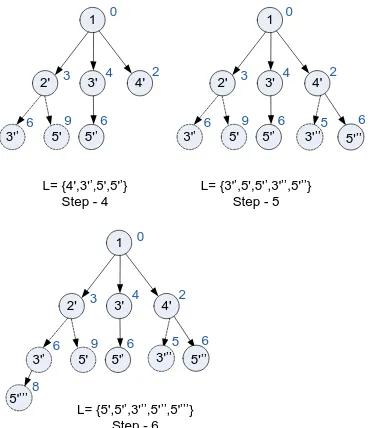
The algorithms start the calculation of K shortest path from the source node s = 1 and form a paths tree rooted at s. A list L is maintained throughout the computation to maintain the node list, which to be visited next by the algorithms. The pictorial explanation describes the re-visitation of nodes by making as-many-as primes with the node number. Total path cost is shown as extra label with every visiting of nodes. The dashed circle and nodes represent calculated path, which is removed later for its higher cost. The algorithms continue with adding nodes (adjacent nodes of the presently visiting node) and labeling relative path (starting from s) to the nodes within the paths tree. The algorithm stops with the condition of L = Φ (no more node is available to visit) and K = 2. The obtained K shortest paths are ranked with K = 1 and K = 2.
[image:2.595.108.224.642.725.2]The final tree of paths rooted at s denotes all the paths computed irrespective of required K. The class of algorithms used to exemplify the computation are proposed by Shier [10,11,12]. These types of algorithms are referred as “Label Correcting” algorithm [20], as labels are corrected (by marking with dashed circles) in a situation of lower cost path available to reach any node. The theoretical complexity is not polynomial for worst case analysis for the particular type of algorithms since it is impossible to establish a polynomial upper bound for the number of labels required for each node in computation time. The “Label correcting” algorithms follow the notion of generalization of the Bellman-Ford-Moore form for the shortest path problem [21,22,23].
3'’
4' 2' 3'
1
5'
L= {4',3'’,5',5'’} Step - 4
0
3 4 2
6 9
5'’ 6
3'’
4' 2' 3'
1
5'
3 4 2
6 9
5'’ 6
L= {3'’,5',5'’,3'’’,5'’’} Step - 5
5 6
3'’
4' 2' 3'
1
5'
3 4 2
6 9
5'’
6 5 6
8
L= {5',5'’,3'’’,5'’’,5'’’’} Step - 6
0
0
3'’’ 5'’’
3'’’ 5'’’
5'’’’
The efficiency of this type of algorithms is improved by manipulating L (the data structure to store node list) in a way as follows in Dijkstra’s algorithm for computing shortest path [24]. The improved class of algorithm is referred as “Label Setting” algorithm in [20]. The “Label Setting” algorithms choose the next node to visit from the node list L, for which the path cost from the source is minimum among all other nodes in L.
3'’
4' 2' 3'
1
5'
3 4 2
6 9
5'’6 5 6 8
L= {5',5'’,3'’’,5'’’,5'’’’} Step - 7
0
3'’’ 5'’’
5'’’’ 5'’’’’7
3'’
4' 2' 3'
1
5'
3 4 2
6 9 5'’
6 5 6
8
L= Φ Step – 8 (Final Step)
0
3'’’ 5'’’
[image:3.595.60.271.172.285.2]5'’’’ 5'’’’’7 K=1 K=2
Fig 4: Last 2 steps of path ranking computation
The improved algorithm become efficient to compute K-shortest paths based on the K-shortest sub paths only, which also excludes the computation of the possible all paths as appear in “Label Correcting” algorithms and hence no correction of labels are required at all.
Dreyfus [8], Martins and Santos [18] and others [5,6,7,17] are propose this form of algorithms. The computational and space complexity of the algorithm is both 𝒪 Km .
4.3
Algorithms based on path deviation
The Optimality Principle asserts that “there is a shortest path formed by shortest sub-paths”, which is further extended for K-shortest path problem. Optimality Principle with K-shortest path problem asserts that the kth shortest path is formed by jth shortest paths, for j ≤ k [20].Yen’s [13] algorithm is designed with direct implementation of the assertion. The algorithm starts with the 1st shortest path π1. To compute the 2nd shortest path π2, the 1st shortest path will be utilized to find out a node vi on the path of π1 such that the cost c s, i + c(i, t) is lowest for all i , and the first edge of the path Pit is not used in the path π1. The special node viis known as “deviation node” and the path pit will be used as deviation path to construct the 2nd shortest path. A path list L is maintained along with the computation to access already computed paths. The algorithm will continue the process of utilizing previous paths to compute the new path.
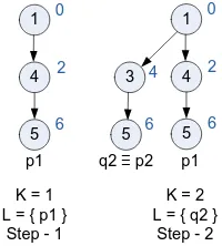
A computational example is shown as figure 5, which uses the input network shown as figure 1 to compute K-shortest paths for K=2.
1
5 4
0
2
6
p1
K = 1 L = { p1 }
Step - 1
1
5 4
0
2
6
p1
K = 2 L = { q2 }
Step - 2 5
3 4
6
[image:3.595.117.217.639.750.2]q2 ≡ p2
Fig 5: Computational example of Yen’s algorithm
The computation starts with the shortest path p1 as shown in step 1. In step 2, the algorithm will search a deviation node on the path p1 to compute a deviation path. Considering node 1 as the deviation node, the resulting deviation paths are calculated as 1-3-5 with path cost 6 and 1-2-5 with path cost 9. So 1-3-5 is the minimum cost deviation path (no lower cost paths are available considering node 4 as deviation node) will be added as the second shortest path p2. The algorithm terminates with K=2. The tree available in step 2 is the K-shortest paths tree rooted at starting node s.
Computational complexity and space complexity of Yen’s algorithm are 𝒪 Kn3 and 𝒪 n2+ Kn respectively [13]. To improve the performance of the algorithm, a shortest paths tree from all nodes to the destination node is useful to provide readily available shortest paths for the calculation of path cost from the deviation node to the destination. A reverse orientation tree is shown as figure 6 formed by shortest paths from all nodes to the destination node.
5
2 1
4 3
5 6
2 4
0
Fig 6: Shortest paths tree in reverse orientation
The computational complexity of Yen’s algorithm reduced to 𝒪 Kn , when the shortest paths tree from all nodes to the destination node is determined separately. Further improvements in computational complexity are observed with the Martin, Pascoal, and Santos’ algorithm [20] and the new implementation of Yen’s algorithm [25] through the support of edge arrangement in sorted forward star form [19] and implicit representation of paths proposed by Eppstein[9].
𝒪 Kn + m log m is the reported improved computational complexity [20] of the newer implementation of the Yen’s algorithm.
5.
COMPARISON OF AVAILABLE
ALGORITHMS
The available algorithms for computing K-shortest paths are compared with their time and space complexity. The comparison is shown as table 1 within the appendix.
6.
APPLICATIONS OF K-SHORTEST
PATHS ALGORITHM
The computation of shortest path included in the situations in which an actual path is desired as output, such as network connection routing, highway and power line engineering, robot motion planning and others. Many optimization problems and complicated matrix searching techniques , such as knapsack problem, construction of optimal inscribed polygon, sequence alignment in molecular biology, length-limited Huffman coding and others can be solved using shortest path problems [9].
community support the typical solution is to compute several shortest paths and then choose the optimum among them considering the criterion.
K-shortest paths computing enable the users to determine the sensitivity of an optimal solution by varying the problem’s parameters. For instance, a biologist can determine the best of an alignment from the available instances of biological sequence alignments generated from more than one shortest paths computation.
7.
CONCLUSION
Current research trend on optimization problem in various domains should be able to incorporate more number of constraints through the use of efficient multiple shortest paths computation methods. This paper emphasizes on K-shortest paths based multiple shortest path computation technique with the detail of the available computationally efficient algorithms.
8.
REFERENCES
[1] Bock, F., Kantner, H. and Haynes, J. 1957 An Algorithm (The rh Best Path Algorithm) for Finding and Ranking Paths Through a Network, Research Report, Armour Research Foundation, Chicago, Illinois, November 15.
[2] Pollack, M. 1961 The k-th Best Route Through a Network, Operations Research, Vol. 9, No. 4, pp. 578-580.
[3] Clarke, S., Krikorian, A. and Rausan, J. 1963 Computing the N Best Loopless Paths in a Network,Jounal of SIAM, Vol. 11, No. 4, pp. 1096-1102.
[4] Sakarovitch, M. 1966 The k Shortest Routes and the k Shortest Chains in a Graph, Operations Research, Center, University of California, Berkeley, Report ORC-32.
[5] Azevedo, J.A., Costa, M.E.O.S., Madeira, J.J.E.R.S., and Martins, E.Q.V. 1993 An algorithm for the ranking of shortest paths. European Journal of Operational Research, 69:97-106.
[6] Azevedo, J.A., Madeira, J.J.E.R.S., Martins, E.Q.V., and Pires, F.M.A. 1990 A shortest paths ranking algorithm, Proceedings of the Annual Conference AIRO'90, Models and Methods for Decision Support, Operational Research Society of Italy, 1001-1011.
[7] Azevedo, J.A., Madeira, J.J.E.R.S., Martins, E.Q.V., and Pires, F.M.A. 994 A computational improvement for a shortest paths ranking algorithm. European Journal of Operational Research, 73:188-191.
[8] Dreyfus, S.E. 1969 An appraisal of some shortest-path algorithms. Operations Research, 17:395-412.
[9] Eppstein, D. 1998 Finding the k shortest paths. SIAM Journal on Computing 28:652-673.
[10]Shier, D. 1974 Computational experience with an algorithm for finding the k shortest paths in a network. Journal of Research of the NBS, 78:139-164.
[11] Shier, D. 1976 Interactive methods for determining the k shortest paths in a network. Networks, 6:151-159.
[12] Shier, D. 1979 On algorithms for finding the k shortest paths in a network. Networks, 9:195-214.
[13] Yen, J.Y. 1971 Finding the k shortest loopless paths in a network. Management Science, 17:712-716.
[14] Martins, E.Q.V., Pascoal, M.M.B., and Santos. J.L.E. 1997 A new algorithm for ranking loopless paths. Research Report, CISUC.
[15] Hoffman, W. and Pavely, R., 1959 A Method for the Solution of the Nth Best Problem, Journal of ACM, Vol. 6, No. 4, pp. 506-514.
[16] Bellman, R. and Kalaba, R 1960 On kth Best Policies, SIAM Journal, Vol. 8, No. 4, pp. 582-588.
[17] Martins, E.Q.V. 1984 An algorithm for ranking paths that may contain cycles. European Journal of Operational Research, 18:123-130.
[18] Martins, E.Q.V. and Santos, J.L.E. 1996 A new shortest paths ranking algorithm. E. Martins and J. Santos. A new shortest paths ranking algorithm. Technical report, Departmentof Mathematics, Universityof Coimbra, (http://www.mat.uc.pt/~eqvm).
[19] Dial, R., Glover, G., Karney, D., and Klingman, D. 1979 A computational analysis of alternative algorithms and labeling techniques for finding shortest path trees. Networks, 9:215-348.
[20] Martins,E. Q. V., Pascoal, M. M. B., and Santos, J. L. E. 1998 The K shortest paths problem. Research Report, CISUC.
[21] Bellman, R.E. 1958 On a routing problem. Quarterly Applied Mathematics, 1:425-447.
[22] Cherkassky, B.V., Goldberg, A.V., and Radzik, T. 1996 Shortest paths algorithms: Theory and experimental evaluation. Mathematical Programming, 73:129-196.
[23] Moore, 1959 E.F. The shortest path through a maze. Proceedings of the International Symposium on the Theory of Switching, Harvard University Press, 285-292.
[24] Dijkstra, E. 1959 A note on two problems in connection with graphs. Numerical Mathematics, 1:395-412.
[25] Martins, E. Q. V. and Pascoal, M. M. B. 2003 A new implementation of Yen’s ranking loopless paths algorithm, 4OR, Springer Berlin, 1:121-133.
Appendix
Table 1. Comparison of available algorithms
Algorithm Type of algorithm Time complexity Space complexity
Bock, Kantner, and Haynes’
Brute-force
Difficult to specify
Pollack’s 𝒪 mK 𝒪 m2+ Km
Sakarovitch’s Difficult to specify
Shier’s Label correcting Difficult to specify
Dreyfus’
Label setting 𝒪 Km 𝒪 Km
Martins and Santos’ 𝒪 Km 𝒪 Km + n
Yen’s
path deviation 𝒪 Kn