Forecasting performance of Logistic STAR exchange rate model: The original and reparameterised versions

Munich Personal RePEc Archive

Forecasting performance of Logistic

STAR exchange rate model: The original

and reparameterised versions

Liew, Venus Khim-Sen and Baharumshah, Ahmad Zubaidi

and Lau, Sie-Hoe

September 2002

Online at

https://mpra.ub.uni-muenchen.de/511/

Forecasting Performance of Logistic STAR Exchange Rate Model: The Original and Reparameterised Versions

Venus Khim-Sen Liewa, Ahmad Zubaidi Baharumshahb, and Sie-Hoe Lauc,*

a

Labuan School of International Business and Finance, Universiti Malaysia Sabah.

b

Department of Economics, Faculty of Economics and Management, Universiti Putra Malaysia.

c

Faculty of Information Technology and Quantitative Science, Universiti Teknologi MARA, Sarawak Campus.

Abstract

Exponential Smooth Transition Autoregressive (ESTAR) model is widely adopted in the exchange rate study as its symmetrical distribution matches that of the symmetrical exchange rate adjustment behaviour. In contrast, another specification of STAR model,

namely the LSTAR (logistic STAR) model is discarded by most researchers in priori in

their exchange rate modeling exercises due to its undesired property of being asymmetry. This study is the first of its kind in examining the validity of this hypothesis that the ESTAR exchange rate model is superior to LSTAR exchange rate model on the basis of forecasting accuracy. Based on the experience of the adjustment process of two nominal exchange rates, we find that the hypothesis is merely theoretical since we fail to provide consistent empirical evidence in favour of the null hypothesis. This warrants us that we need not be too pessimistic on the usage of LSTAR model in exchange rate study. In our effort to rekindle the usage of LSTAR model, we further reparameterized the original version into the so-called absolute version, which has symmetrical distribution properties, in accordance with the well-known symmetrical adjustment process of exchange rate. The resulting ALSTAR model has proven to be a more promising model in the sense that it has improved significantly from its original version as well as the ESTAR model, which has thus far been deemed the most appropriate nonlinear exchange rate model.

JEL Classification: F31, C53

Keywords: LSTAR, ESTAR, forecasting accuracy, nonlinear, exchange rate

Forecasting Performance of Logistic STAR Exchange Rate Model: The Original

and Reparameterised Versions

1. Introduction

A number of empirical studies have documented that exchange rate behavior may be well

characterized by the Smooth Transition Autoregressive (STAR) process (Taylor and

Sarno, 1998; Sarantis, 1999; Taylor and Peel, 2000; Sarno, 2000; Baum et al., 2001;

Guerra, 2001; Liew et al., 2004). STAR model is a nonlinear econometric model that is

able to capture the movement of exchange rate, which adjusts every moment but the

speed of adjustment varies with the size of exchange rate deviations. The STAR model

for a mean corrected variable of interest, z_t−d may be parameterized as:

t

z = ∑

= − p

1 i i t i

z

β + (∑

= − p

1 i i t i

z *

β )F(z_t−d) + εt (1)

whereβi and

*

i

β , i = 1, …, p are autoregressive parameters, F(·) is the transition

function depending on the lagged level, z_t−d where d is known as the delay length or

delay parameter, and εt is a white noise with zero mean and constant variance.

Two forms of transition function given in Teräsvirta (1994) are the logistic function

and the exponential function

F(z_t−d) = 1 – exp[–γ 2(z_t−d)2] (3)

where γ2stands for the transition parameter, which measures the speed of adjustment.

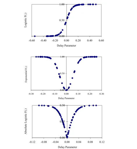
A plot of these typical transition functions with respect to the delay parameter is depicted

in Figure 1. It is clear from the Figure 1 that logistic transition function has a S shape

distribution (top panel), while exponential transition function has symmetrical

inverted-bell shape distribution (middle panel). Note that values of these functions lie between 0

and 1; see Teräsvirta (1994) for theoretical issues on these functions.

STAR model (1) with specification (2) is known as ESTAR or exponential STAR model,

whereas with specification (3) is termed LSTAR or logistic STAR model. These two

models have quite different empirical implication of dynamic exchange rate behaviour.

The LSTAR model describes the asymmetrical nonlinear adjustment process, while the

ESTAR model suggests symmetrical nonlinear adjustment process (Sarantis, 1999).

LSTAR is a monotonic increasing function of z_t−dand yields asymmetric adjustment

towards equilibrium (top panel, Figure 1). However, the theoretically assumption that

exchange rate adjustment is symmetric implies LSTAR model as inappropriate for

ESTAR model as the correct represent of exchange rate (for instance, Taylor and Peel;

2000 and Sarno, 2000)1. In order to revitalize the use of LSTAR model, we propose to

reparameterize LSTAR model, with logistic function specified as

F(z_t−d) = [1 + exp(_-γ 2|z_t−d|)]-1_-½ (4)

where | · | implies absolute value.

We refer to the resulting model as ALSTAR (absolute LSTAR) to differentiate it from

the original specification (2). The absolute logistic transition function (4) allows a

V-shaped (similar to inverted bell-V-shaped, but with sharp vertex) symmetry adjustment

process of the exchange rate towards the mean of z_t that is zero in our case. This logistic

F(·) is bounded between zero and one-half, with F(·) → 0 when γ 2→ 0 and F(·) → ½

when γ 2→∞. The plot of our proposed absolute transition function is given in the lower

panel of Figure 1. The V shape distribution, with values between 0 and 0.5 are explicitly

shown in Figure 1. We will show later, that this specification of LSTAR is also capable

of describing the symmetrical behavior in exchange rates.

1

0.00 0.50 1.00

-0.60 -0.40 -0.20 0.00 0.20 0.40 0.60

Delay Parameter

Logistic F(.)

0.00 0.50 1.00

-0.30 -0.20 -0.10 0.00 0.10 0.20 0.30

Delay Parameter

Exponential F(.)

Note: Values in the plots are hypothetical.

Figure 1: Theoretical shapes of various transition functions 0.00

0.25 0.50

-0.12 -0.08 -0.04 0.00 0.04 0.08 0.12

Delay Parameter

The objectives of this paper are: First, to evaluate the forecasting performance of LSTAR

model with respect to the ESTAR model. With this approach, effectively we are

providing a platform to examine how far the hypothesis that ESTAR model is more

relevant in characterizing the exchange rate adjustment process than the LSTAR model

could be justified. Second, to evaluate our proposed ALSTAR model using linear

autoregressive (AR) model, LSTAR model and ESTAR model as benchmark. These

objectives could be accomplished based on the mean square error (MSE) and the

robustness of this criterion is subjected to Meese and Rogoff (1988) test.

This paper proceeds as follows. Our research methodology is described in Section 2,

whereas results of this study and discussions are presented in Section 3. Our conclusions

are given in the final section.

2. Methodology

Data

The data employed in this study includes yen-based nominal exchange rates (domestic

price of foreign money) and relative prices (proxied by the ratio consumer price indices).

Quarterly data series from two ASEAN neighboring countries, namely Malaysia and

Thailand are collected from the International Financial Statistics, published by

International Monetary Fund. Our sample period ranges from 1980:1 to 2001:2. The

for model estimation, while the rest are kept for assessing the out-sample forecast

performance of the studied models.

Standard augmented Dickey Fuller unit root has been performed on these data and results

(available upon request) reveal that they are all integrated of order one. In addition, the

exchange rates involved are found cointegrated with their respectively relative prices

(ratio of domestic price to foreign price) based on the commonly used Johensen and

Juselius procedure (available upon request). This is supportive of the long run purchasing

power parity hypothesis, which implies that exchange rates adjust towards their

equilibrium Purchasing Power Parity (PPP) values in the long run, although deviations

may occur due to transaction costs in the short run (Dumas, 1992). The theoretical

no-arbitrage model of Dumas that exchange rates adjustment are nonlinear in nature may be

tested by performing the linearity test of as described in Luukkonen et al. (1988) on the

deviations (in this study, z_t) of exchange rate, from the equilibrium level.

Linearity Test

We employ auxiliary regression of the following specification

t

z = α₀ + p( * _{t i t d i}* _{t t}2_d)

1

i i t d i

z z z

z

z _{− − −}

= − + +

∑ α α δ + *τ z_t3_−d+ω_t (5)

The null hypothesis to be tested is that

0

H : * *

i i δ

where the optimal lag length, p and the delay parameter, d have to be determined in

advance2. This null hypothesis may be tested using the Lagrange Multiplier (LM) type

test statistic as described in Luukkonen et al. (1988); see Teräsvirta (1994) also.

Rejection of null hypothesis (6) implies exchange rate adjusts nonlinearly as

characterized by the STAR. One may proceed on a subset of tests if the objective is to

check whether LSTAR or ESTAR is the correct specification. Nonetheless, there is a

possibility that both models are appropriate. In such case, Escribano and Jorda (2001)

suggest to choose the one with smaller marginal significance value of LM statistic.

However, the selection may be postponed to the final stage of model evaluation via

certain criteria (Teräsvirta, 1994). This study focuses on forecasting performance; hence,

the chose of model specification is not our concern here.

Forecasting performance criteria

The overall in-sample (65 quarterly observations) and out-sample performance of the

estimated absolute LSTAR model over the forecast horizon of n =14 over the period

1997:3 to 2000:4 are evaluated by taking the linear AR (p) and ESTAR models as the

benchmark3. The criterion involved is the ratio of forecast error measured in mean square

error (MSE), with the forecast error of benchmark model as denominator. We compute

the Meese and Rogoff (1988) MR statistic to check the statistical significance of the MSE

criteria. MR for finite sample is given by

2

Following Liew et al. (2004), p is determined by AICC, the Akaike information criterion (biased

corrected version) and for 1≤d≤12, the optimal value is the one that provides the smallest marginal

significance value of the LM test statistic.

3

MR =

∑

∼

N (0, 1) (7)

where U and V are transformed functions of forecast errors of two rival models; sUV is

the sample covariance of means of U and V and is approximated by

) ( )

(u u v v

n 1 j n 1 j

j − −

∑

=

where

∑

= = n 1 j j u n 1

u and

∑

= = n 1 j j v n 1

v with u_j =e_1j−e_2jand

j 2 j 1 j e e

v = + in which e_ij, i = 1, 2 is the jth forecast error of model i; and n is the number

of forecasts.

The null hypothesis of MR statistic, which states that cov (U, V) = 0 implies evaluating

whether MSE1 = MSE2. If MR statistics is significantly different from the critical values

(from Z table if n is large enough, t table otherwise), the improving in forecasting

accuracy in model 1 over model 2 in the MSE ratio will then be statistically significant.

3. Results and Discussions

Linearity Test

The results of linearity tests suggest that the null of linearity has been rejected, at

standard significance levels, in favor of both the LSTAR and ESTAR specifications.4

4

Thus LSTAR model with p = 1 and d = 4 is an appropriate representation of the ringgit

adjustment process. One the other hand, this series could be characterized by ESTAR

model with p = 1 and d = 2 as well. As for the adjustment of the baht, it is described by

both LSTAR model with p = 3 and d = 1 and ESTAR model with p = 3 and d = 5.

Residual diagnostic by the Ljung Box portmanteau Q statistic shows that all models are

free from serial correlation, which is normally associated with autoregressive model.

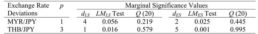
These results are summarized in Table 1.

Table 1

Linearity Test Results

Marginal Significance Values Exchange Rate

Deviations

p

dLS LMLS Test Q (20) dES LMESTest Q (20)

MYR/JPY 1 4 0.056 0.219 2 0.025 0.445

THB/JPY 3 1 0.016 0.579 5 0.001 0.995

Notes: Lagrange Multiplier (LM) test tests for the null hypothesis of H0: Linear model is

correct. Rejection of H0 by the LMLS (LMES Test) test implies the presence of nonlinearity

in favour of LSTAR (ESTAR) model. dLS(dLS) stands for optimal delay lag length that

minimizes the marginal significance value of LMLS (LMES) test. Ljung-Box Q statistic [Q

(20)] detects the presence of serial correlation in the model’s residuals up to 20 lags, if any.

Estimated Models

The estimated models are tabulated in Table 2. As serial correlation is a major problem in

any time series model, we include the Ljung Box Portmanteau (Q) test to detect the

presence of serial correlation. The p-values of these Q statistics indicate that all estimated

characterizing the adjustment process of MYR/JPY and THB/JPY towards the long-run

PPP equilibrium. As a measure to check whether the nonlinear specification is correct,

we employ the overall significance F test. The null hypothesis of this F test is that the

linear specification is correct. Results show that the joint effect of the nonlinear

parameters and the transition parameter in each model is significance at standard levels,

indicating that the linear specification has been rejected in favour of the STAR

specification. In addition, we find that STAR model yields smaller variance than their

linear counterpart, indicating that it potential to produce smaller forecast error than the

AR model (Teräsvirta and Anderson, 1993). The last two finding confirms that the

adjustment process of MYR/JPY and THB/JPY towards the long-run PPP equilibrium is

of nonlinear nature. Thus, this study has provided further empirical evidence on the

existence of the nonlinear dynamic in the context of ASEAN foreign exchange market, in

accordance to Lim et al. (2002).

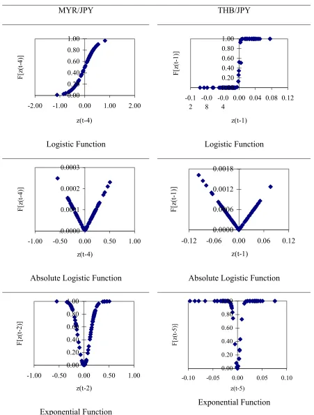
The empirical distributions of various transition functions are given in Figure 2. The top

panel depicts the logistic functions for the MYR/JPY (left) and THB/JPY (right) rates.

This function is a monotonic increasing function of exchange rate deviations as expected,

with speed of transition varies across exchange rates. In particular, the MYR/JPY

adjustment is a smooth and steady process, whereas the THB/JPY adjustment is speedy

and abrupt. The V shape distribution of absolute transition function is plotted at the

middle panel of Figure 2. This figure shows that there are satisfactorily equal amount of

negative and positive adjustments around the equilibrium level (indicated by the zero

process of exchange rates could be well characterized by the absolute LSTAR model.

Finally, the empirical distributions of exponential functions, which are in line with most

related studies, are given in the bottom panel of Figure 2. This is not surprising, as it has

been well documented that this function fitted the symmetrical adjustment of exchange

Table 2

Estimated STAR Models

LSTAR Model Absolute LSTAR

Model

ESTAR Model Paramet

er MYR/JPY THB/JPY MYR/JPY THB/JPY MYR/JPY THB/JPY

1

β _0.85×100

(0.13×100)

a

–0.57×104

(0.67×101)

b

–0.11×101

(0.11×100)

a

0.15×101

(0.22×100)

a

0.14×101

(0.35×101)

0.22×101

(0.77×100)

a

2

β _{–– 0.30×10}5

(0.10×105)

b

–– –0.20×10

-1

(0.35×101)

b

–– 0.10×10-1

(0.10×10

-4

)a

3

β _{–– –0.23×10}5

(0.96×104)

b

–– 0.20×100

(0.25×101)

–– –0.01×10

-1 (0.10×10 -4 )a * 1

β –0.10×10

-1

(0.14×100)

0.11×105

(0.12×105)

–0.14×104

(0.10×104)

–0.16×103

(0.25×103)

–0.60×100

(0.35×101)

–0.13×101

(0.76×100)

b

*

2

β –– –0.61×105

(0.20×105)

b

–– –0.10×104

(0.63×103)

–– –0.16×101

(0.69×100)

*

3

β –– 0.47×105

(0.19×105)

b

–– 0.73×103

(0.53×103)

–– –0.40×10

-2

(0.46×10

-1

)

2

γ 0.44×101

(0.10×10

-4

)a

0.17×103

(0.49×102)

b 0.18×10-3 (0.10×10 -4 )a 0.60×10-1 (0.10×10 -4 )a 0.39×102

(0.35×101)

a

0.27×103

(0.11×101)

a

Diagnostic Checkings

VNL/VL 0.959 0.932 0.968 0.813 0.883 0.837

p (F test)

0.060 0.024 0.039 0.017 0.030 0.011

p (Q test)

0.262 0.876 0.264 0.969 0.303 0.987

Notes: Figures in parentheses are standard errors of estimated parameters. Superscript a

and b imply significant at 5% and 10% respectively. VNL/VL stands for ratio of residual

variance of nonlinear model to that of linear model. p (·) stands for p-value of the implied

MYR/JPY THB/JPY 0.00 0.20 0.40 0.60 0.80 1.00

-2.00 -1.00 0.00 1.00 2.00

z(t-4) F[z(t-4)] Logistic Function 0.00 0.20 0.40 0.60 0.80 1.00 -0.1 2 -0.0 8 -0.0 4

0.00 0.04 0.08 0.12

z(t-1) F[z(t-1)] Logistic Function 0.0000 0.0001 0.0002 0.0003

-1.00 -0.50 0.00 0.50 1.00

z(t-4)

F[z(t-4)]

Absolute Logistic Function

0.0000 0.0006 0.0012 0.0018

-0.12 -0.06 0.00 0.06 0.12

z(t-1)

F[z(t-1)]

Absolute Logistic Function

0.00 0.20 0.40 0.60 0.80 1.00

-1.00 -0.50 0.00 0.50 1.00

z(t-2)

F[z(t-2)]

Exponential Function

Exponential Function

Figure 2: Plots of estimated transition functions

0.00 0.20 0.40 0.60 0.80 1.00

-0.10 -0.05 0.00 0.05 0.10

z(t-5)

Forecast Accuracy

Our first forecasting accuracy comparison exercise is done using AR model as

benchmark. By observing the MSE ratio, it is clear that all the nonlinear STAR models

have out-predicted the linear AR models in the context of in-sample forecasting (Table

3). This finding is not by chance as the MR statistic has verified that it is significant at

10% or better. One implication of this finding is that STAR model, rather than the

conventional AR model could better explain the past exchange rate behavior. We note

here that apart form being able to explain the past, a good model should also have the

ability to predict the future with satisfactory accuracy. This scenario is observed in a

number of related studies and is once again experienced in this current study5. More

specifically, we find that none of the outstanding performance of LSTAR models (for

MYR/JPY and THB/JPY) can be extended to the out-sample horizon6. As for the ESTAR

model, results are mixed: The ESTAR MYR/JPY model does continue to be more

excellence than its linear counterpart, but the ESTAR THB/JPY model shows reverse

result. Meanwhile, the ALSTAR model seems to be the only promising model that carries

over its outstanding forecasting ability from the in-sample horizon to the out-sample

horizon. This conclusion is drawn from the fact that ALSTAR model remains the only

model that out-predicted its linear counterpart significantly in predicting both the future

behavior of MYR/JPY and THB/JPY adjustments. Hence, while LSTAR model has been

5

For instance, Choo and Ahmad 1999; Tashman, 2000; Liew and Shitan, 2002 documented that models that explained the past best need not necessarily be the best forecasting model.

6

discarded, in the past, due to its inabilities to characterize the symmetrical exchange rate

adjustment behavior, this study has provided an improved version, namely the absolute

LSTAR model, which forecasting performance has been proven promising. This claim

will be more obvious by conducting the next exercise.

Table 3

Overall Forecasting Accuracy with AR as Benchmark

MSE Ratio (MR Test Statistics)

Exchange Rate

LSTAR / AR ALSTAR / AR ESTAR / AR

In-Sample (65 quarters)

MYR/JPY 0.929 (1.978)b 0.146 (1.845)b 0.429 (1.541)b

THB/JPY 0.399 (1.520)a 0.381 (1.477)a 0.523 (1.569)b

Out-Sample (14 quarters)

MYR/JPY 1.008 (4.132)b 0.382 (6.707)b 1.562 (5.561)b

THB/JPY 1.104 (7.721)b 0.438 (6.466)b 0.588 (6.385)b

Notes: MR tests the null hypothesis of “equal accuracy” against two-sided alternative of

“unequal accuracy” in terms of MSE ratio. The 10%, 5% and 1% critical values are

2.326, 1.645 and 1.282 respectively.Superscripts a and b denote significant at 10% and

5% level or better, respectively.

The second forecasting accuracy comparison exercise aims is done within the context of

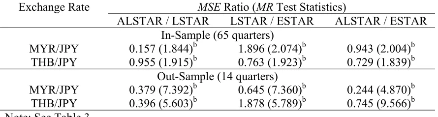
various STAR models. The results of comparison are tabulated in Table 4. From Table 4,

the original version of LSTAR model is at most comparable to the ESTAR model in both

the in- and out-sample forecasting horizons. Table 4 also reveals that absolute version of

LSTAR has significantly improved over its original version, in all forecasting horizons.

This finding is not surprising since the former, but not the latter could account for

well-documented symmetrical exchange rate adjustment. Our most striking result is that

model in the sense that ALSTAR model has shown its potential in predicting the future

exchange rate adjustment behavior (as far as MYR/JPY and THB/JPY is concerned) with

better accuracy than the ESTAR model, apart from giving better explanation for the past

adjustment.

Table 4

Comparison of Overall Forecasting Accuracy among STAR Models

MSE Ratio (MR Test Statistics)

Exchange Rate

ALSTAR / LSTAR LSTAR / ESTAR ALSTAR / ESTAR

In-Sample (65 quarters)

MYR/JPY 0.157 (1.844)b 1.896 (2.074)b 0.943 (2.004)b

THB/JPY 0.955 (1.915)b 0.763 (1.923)b 0.729 (1.839)b

Out-Sample (14 quarters)

MYR/JPY 0.379 (7.392)b 0.645 (7.360)b 0.244 (4.870)b

THB/JPY 0.396 (5.603)b 1.878 (5.789)b 0.745 (9.566)b

Note: See Table 3.

4. Conclusions

The advanced econometric STAR model has been widely applied in the exchange rate

study due to its capability in characterizing the nonlinear exchange rate adjustment

behaviour. To date, two specifications, namely the LSTAR (logistic STAR) and the

ESTAR (exponential STAR) have thus far been proposed. The latter is preferable since

its symmetrical distribution matches that of the symmetrical exchange rate adjustment

behaviour. In contrast, most researchers discard the former in priori in their exchange

rate modeling exercises due to its undesired property of being asymmetry. Nevertheless,

to date, not a single published article has provided empirical evidence on the hypothesis

the basis of forecasting accuracy. Based on the experience of the adjustment process of

two nominal exchange rates, we fail to provide consistent results in favour of the null

hypothesis. This warrants us that we need not be too pessimistic on the usage of LSTAR

model in exchange rate study. In our effort to rekindle the usage of LSTAR model, we

further reparameterized the original version into the so-called absolute version, which has

symmetrical distribution properties, in accordance with the well-known symmetrical

adjustment process of exchange rate. The resulting ALSTAR model has proven to be a

more promising model in the sense that it has improved significantly from its original

version as well as the ESTAR model, which has thus far been deemed the most

appropriate nonlinear exchange rate model.

References

Baum, C. F., Barkoulas, J. T. and Caglayan, M., 2001. Nonlinear adjustment to

Purcahsing Power Parity in the Post-Bretton Woods era. Journal of International

Money and Finance. 20: 379–399.

Choo, W. C. and Ahmad, I. M. 1999. Performance of GARCH models in Forecasting

Stock Market Volality. Journal of Forecasting. 18: 333 – 343.

Dumas, B. 1992. Dynamic equilibrium and the real exchange rate in a spatially seperated

Escribano, A and Jorda, O. 2001. Testing Nonlinearity: Decision Rules for Selecting

between Logistic and Exponential STAR models. Spanish Economic Review. 3: 193 –

209.

Guerra, R. 2001. Nonlinear Adjustment towards Purchasing Power Parity: The Swiss

Franc – German Case. Working Paper. Department of Economics, University of

Geneva, Geneva.

Luukkonen, R. Saikkonen, P. and Teräsvirta, T. 1988. Testing linearity against Smooth

Transition Autoregressive Models. Biometrika. 75: 491– 499.

Meese, R. A. and Rogoff, K. 1988. Was Is Real? The Exchange Rate-Interest Differential

Relation over the Modern Floating Rate Period. Journal of Finance. 43: 933 – 948.

Liew, V. K. S., Baharumshah, A. Z. and Lau, E. 2004. Nonlinear Adjustment to

Purchasing Power Parity in ASEAN Exchange Rates. ICFAI Journal of Applied

Economics. 3(6): 7 – 18.

Liew, K. S. and Shitan, M. 2002. The Performance of AICC as Order Determination

Criterion in the Selection of ARMA Time Series Models. Pertanika Journal of

Science and Technology. 10(1): 25 – 33.

Lim, K. P. , Mohamed, A. and Habibullah, M. S. 2002. Non-linear Dependence in

ASEAN-5 Foreign Exchange Rates. Proceeding of Asian Pacific Economics and

Business Conference, 2nd – 4th October, 2002, Kuching, Sarawak, Malaysia.

Sarantis, N. 1997. Modeling Non-linearities in Real Effective Exchange Rates. Journal of

International Money and Finance. 18: 27 – 45.

Sarno, L. 2000. Real exchange rate behaviour in high inflation countries: empirical

Tashman, L. J. 2000. Out-of-sample Tests of Forcasting Accuracy: An Analysis and

Review. International Journal of Forecasting. 16: 437 – 450.

Taylor, M. P. and Peel, D. A. 2000. Nonlinear adjustment, long-run equilibrium and

exchange rate fundamentals. Journal of International Money and Finance. 19: 33 –

53.

Taylor, M. P. and Sarno, L. 1998. The behaviour of real exchange rates during the

post-Bretton Wood period, Journal of International Economics, 46, 261 – 312.

Teräsvirta, T. 1994. Specification, estimation, and evaluation of Smooth Transition

Autoregressive Models. Journal of the American Statistical Association. 89(425):

208–218.

Teräsvirta, T. and Anderson, H. M. 1993. Characterizing nonlinearities in business

cycles using Smooth Transition Autoregressive Models. In in M. H. Pesaran & S.

M. Potter (eds.) Nonlinear Dynamics, Choas and Econometrics. US: John Wiley.

pp. 111–128.

Tong, H. and Lim. K. S. 1980. Threshold Autoregression, limit cycles and cyclical data.