Using Genetic Algorithms to Develop Strategies for the Prisoners Dilemma

Using Genetic Algorithms to Develop

Strategies for the Prisoners Dilemma

Haider, Adnan

Department of Economics, Pakistan Institute of Development

Economics, Islamabad

12 November 2005

Online at

https://mpra.ub.uni-muenchen.de/28574/

1

FOR THE PRISONER’S DILEMMA

ADNAN HAIDER

PhD Fellow Department of Economics Pakistan Institute of Development Economics

Islamabad, Pakistan.

The Prisoner‘s Dilemma, a simple two-person game invented by M errill Flood & M elvin Dresher in the 1950s, has been studied extensively in Game Theory, Economics, and Political Science because it can be seen as an idealized model for real-world phenomena such as arms races (A xelrod

1984). In this paper, I describe a GA to search for strategies to play the Iterated Prisoner‘s

Dilemma, in which the fitness of a strategy is its average score in playing 100 games with itself and with every other member of the population. Each strategy remembers the three previous turns with a given player, by using a population of 20 strategies, fitness-proportional selection, single-point crossover with Pc=0.7, and mutation with Pm=0.001.

JEL Classifications: C63, C72

Keywords: GA, Crossover, M utation and Fitness-proportional.

1. Introduction

The Prisoner's Dilemma, can be formulated as follows: Two individuals (call them Mr. X and Mr. Y) are arrested for committing a crime together and are held in separate cells, with no communication possible between them. Mr. X is offered the following deal: If he confesses and agrees to testify against Mr. Y, he will receive a suspended sentence with probation, and Mr. Y will be put away for 5 years. However, if at the same time Mr. Y confesses and agrees to testify against Mr. X, his testimony will be discredited, and each will receive 4 years for pleading guilty. Mr. X is told that Mr. Y is being offered precisely the same deal. Both Mr. X and Mr. Y know that if neither testifies against the other they can be convicted only on a lesser charge for which they will each get 2 years in jail. Should Mr. X "defect" against Mr. Y and hope for the suspended sentence, risking, a 4-year sentence if Mr. Y defects? Or should he "cooperate" with Mr. Y (even though they cannot communicate), in the hope that he will also cooperate so each will get only 2 years, thereby risking a defection by Mr. Y that will send him away for 5 years?

The game can be described more abstractly. Each player independently decides which move to make— i.e., whether to cooperate or defect. A "game" consists of each player's making a decision (a "move"). The possible results of a single game are summarized in a payoff matrix like the one shown in table 1.1. Here the goal is to get as many points (as opposed to as few years in prison) as possible. (In table 1.1, the payoff in each case can be interpreted as 5 minus the number of years in prison.) If both players cooperate, each

____________________________________________

gets 3 points. If player A defects and player B cooperates, then player A gets 5 points and player B gets 0 points, and vice versa if the situation is reversed. If both players defect, each gets 1 point. What is the best strategy to use in order to maximize one's own payoff? If you suspect that your opponent is going to cooperate, then you should surely defect. If you suspect that your opponent is going to defect, then you should defect too. No matter what the other player does, it is always better to defect. The dilemma is that if both players defect each gets a worse score than if they cooperate. If the game is iterated (that is, if the two players play several games in a row), both players always defecting will lead to a much lower total payoff than the players would get if they cooperated.

Table 1. The Payoff M atrix

Player A

Cooperate Defect

Player B

Cooperate 3, 3 0, 5

Defect 5, 0 1, 1

Assume a rational player is faced with playing a single game (known as one -shot) of the Prisoner's Dilemma described above and that the player is trying to maximize their reward. If the player thinks his/her opponent will cooperate, the player will defect to receive a reward of 5 as opposed to cooperation, which would have earned him/her only 3 points. However if the player thinks his/her opponent will defect, the rational choice is to

also defect and receive 1 point rather than cooperate and receive the sucker‘s payoff of 0

points. Therefore the rational decision is to always defect.

But assuming the other player is also rational he/she will come to the same conclusion as the first player. Thus both players will always defect; earning rewards of 1 point rather than the 3 points that mutual cooperation could have yielded. Therein lays the dilemma. In game theory the Prisoner's Dilemma can be viewed as a two players, non zero-sum and simultaneous game. Game theory has proved that always defecting is the dominant strategy for this game (the Nash Equilibrium). This holds true as long as the payoffs follow the relationship T > R > P > S, and the gain from mutual cooperation is greater than the average score for defecting and cooperating, R > (S + T)/ 2. While this game may seem simple it can be applied to a multitude of real world scenarios. Problems ranging from businesses interacting in a market, personal relationships, super power

negotiations and the trench warfare ―live and let live‖ system of World War I have all

been studied using some form of the Prisoner's Dilemma.

2. Iterated Prisoner’s Dilemma

the above discussion of the Prisoner's Dilemma the dominant mutual defection strategy relies on the fact that it is a one-shot game, with no future. The key to the IPD is that the two players may play each other again; this allows the players to develop strategies based

on previous game interactions. Therefore a player‘s move now may affect how his/her

opponent behaves in the future and thus affect the player‘s future payoffs. This removes the single dominant strategy of mutual defection as players use more complex strategies dependant on game histories in order to maximize the payoffs they receive. In fact, under the correct circumstances mutual cooperation can emerge. The length of the IPD (i.e. the number of repetitions of the Prisoner's Dilemma played) must not be known to either player, if it was the last iteration would become a one-shot play of the Prisoner's Dilemma and as the players know they would not play each other again, both players would defect. Thus the second to last game would be a one-shot game (not influencing any future) and incur mutual defection, and so on till all games are one-shot plays of the Prisoner's Dilemma.

This paper is concerned with modeling the IPD described above and devising strategies to play it. The fundamental Prisoner's Dilemma will be used without alteration. This assumes a player may interact with many others but is assumed to be interacting with them one at a time. The players will have a memory of the previous three games only (memory-3 IPD).

3. Genetic Algorithms

Genetic Algorithms are search algorithms based on the mechanics of natural selection and natural genetics. John Holland at the University of Michigan originally developed them. They usually work by beginning with an initial population of random solutions to a given problem. The success of these solutions is then evaluated according to a specially

designed fitness function. A form of ‗natural selection‘ is then performed whereby

solutions with higher fitness scores have a greater probability of being selected. The

selected solutions are then ‗mated‘ using genetic operators such as crossover and

mutation. The children produced from this mating go on to form the next generation. The theory is that as fitter genetic material is propagated from generation to generation the solutions will converge towards an optimal solution. This research utilizes Genetic Algorithms to develop successful strategies for the Prisoner's Dilemma.

A simple GA works on the basis of the following steps:

Step 1.

Start with a randomly generated population of n l-bit chromosomes (Candidate solution to a problem).

Step 2.

Calculate the fitness f(x) of each chromosome x in the population.

Step 3.

o _{Select a pair of parent chromosomes from the current population, the}

probability of selection being an increasing function of fitness. Selection

is done ―with replacement‖ meaning that, the same chromosome can be selected more than once to become a parent.

o _{With probability Pc} (the ―crossover probability‖), crossover the pair at a

randomly chosen point to form two offspring. If no crossover takes place, form two offspring that are exact copies of their respective parents. (Note: crossover may be in ―single point‖ or ―multi-point‖ version of the GA.)

o _{Mutate the two offspring at each locus with probability Pm (the mutation}

probability or mutation rate), and place the resulting chromosomes in the new population. (Note: if n is odd, one new population member can be described at random.)

Step 4.

Replace the current population with the new population.

Step 5.

Go to step 2.

4. Experimental Setup

Genetic Algorithms provide the means by which strategies for the Prisoner's Dilemma are developed in this paper. As this is the principal objective of the research, naturally the genetic algorithm used is one of the systems major components. The other system components have been designed to suit the Genetic Algorithm. As such, in describing the genetic algorithms implementation most of the other components will also be described. What follows is a description of how a genetic algorithm was implemented to evolve strategies to play the Iterated Prisoner's Dilemma.

4.1. Figuring out Strategies

The first issue is figuring out how to encode a strategy as a string. Suppose the memory of each player is one previous game. There are four possibilities for the previous game:

Case 1: CC

Case 2: CD

Case 3: DC

Case 4: DD

Where C denotes ―cooperate‖ and D denotes ―defect‖. Case I is when both players

cooperated in the previous game, case II is when player A cooperated and player B defected, and so on.

If CC (Case 1) Then C If CD (Case 2) Then D If DC (Case 3) Then C If DD (Case 4) Then D

If the cases are ordered in this canonical way, this strategy can be expressed compactly as the string CDCD. To use the string as a strategy, the player records the moves made in the previous game (e.g., CD), finds the case number i by looking up that case in a table of ordered cases like that given above (for CD, i = 2), and selects the letter in the ith

position of the string as its move in the next game (for i = 2, the move is D). Consider the tournament involved strategies that remembered three previous games, then there are 64 possibilities for the previous three games:

CC CC CC (Case 1),

CC CC CD (Case 2),

CC CC DC (Case 3),

… … … … … … … … … … … …

i

… … … … … … … … … … … …

DD DD DC (Case 63)

DD DD DD (Case 64)

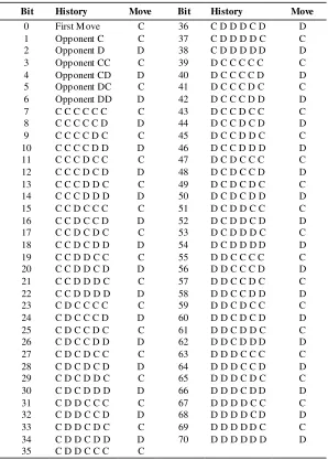
Thus, a 64-letter string, e.g., CCDCDCDCDCDC… can encode a strategy. Since using the strategy requires the results of the three previous games, we can use a 70-letter string, where the six extra letters encoded three hypothetical previous games used by the strategy to decide how to move in the first actual game. Since each locus in the string has two possible alleles (C and D), the number of possible strategies is 270_{. The search space} is thus far too big to be searched exhaustively.

The history in table 2 is stated in the order Your first move, Opponents first Move, Your second move, Opponents second Move, Your third move, Opponents third Move. The move column indicates what move to play for the given history. Table 2 also shows how the TFT strategy is encoded using this scheme. The resulting TFT chromosome is:

CCDCDCDCDCDCDCDCDCDCDCDCDCDCDCDCDCDCDCDCDCDCDCDCDCD CDCDCDCDCDCDCDCDCDCDCDCDCDCDCDCDCDCDCDCDCDCDCDCDCDC DCDCDCDCDCDCDCDCDCDCDCDCDCDCDCDCD

110101010101010101010101010101010101010101010101010101010101010101010101 010101010101010101010101010101010101010101010101010101010101010

Table 1. Encoding Strategies.

Bit History Move Bit History Move

0 First M ove C 36 C D D D C D D

1 Opponent C C 37 C D D D D C C

2 Opponent D D 38 C D D D D D D

3 Opponent CC C 39 D C C C C C C

4 Opponent CD D 40 D C C C C D D

5 Opponent DC C 41 D C C C D C C

6 Opponent DD D 42 D C C C D D D

7 C C C C C C C 43 D C C D C C C

8 C C C C C D D 44 D C C D C D D

9 C C C C D C C 45 D C C D D C C

10 C C C C D D D 46 D C C D D D D

11 C C C D C C C 47 D C D C C C C

12 C C C D C D D 48 D C D C C D D

13 C C C D D C C 49 D C D C D C C

14 C C C D D D D 50 D C D C D D D

15 C C D C C C C 51 D C D D C C C

16 C C D C C D D 52 D C D D C D D

17 C C D C D C C 53 D C D D D C C

18 C C D C D D D 54 D C D D D D D

19 C C D D C C C 55 D D C C C C C

20 C C D D C D D 56 D D C C C D D

21 C C D D D C C 57 D D C C D C C

22 C C D D D D D 58 D D C C D D D

23 C D C C C C C 59 D D C D C C C

24 C D C C C D D 60 D D C D C D D

25 C D C C D C C 61 D D C D D C C

26 C D C C D D D 62 D D C D D D D

27 C D C D C C C 63 D D D C C C C

28 C D C D C D D 64 D D D C C D D

29 C D C D D C C 65 D D D C D C C

30 C D C D D D D 66 D D D C D D D

31 C D D C C C C 67 D D D D C C C

32 C D D C C D D 68 D D D D C D D

33 C D D C D C C 69 D D D D D C C

34 C D D C D D D 70 D D D D D D D

35 C D D C C C C

4.2. Fitness Function

avg avg avg avg

f

f

f

c

f

f

b

(

(

))

objects in some form of IPD. The Game object was implemented to play a game of IPD for a specified number of rounds between two players. This object simply keeps track of

two Prisoner‘s scores and game histories while asking them for new moves until the rounds limit is met. The tournament object uses this class to organize a round robin IPD

tournament, akin to Axelrod‘s [1] computer tournaments. In such a tournament an array of Prisoner‘s is supplied as the population and every Prisoner plays an IPD Game against

every other Prisoner and themselves. Each player‘s payoff after these interactions have completed is deemed to be the player‘s fitness score.

4.3. Fitness Scaling

The fitness scores calculated above will serve to determine which players go on to

reproduce and which players ‗die off‘. However these ‗raw‘ fitness values present some

problems. The initial populations are likely to have a small number of very high scoring individuals in a population of ordinary colleagues. If using fitness proportional selection, these high scorers will take over the population rapidly and cause the population to

converge on one strategy. This strategy will be a mixture of the high scorers‘ strategies,

however as the population did not get time to develop these strategies may be sub-optimal, and the population will have converged prematurely. In the later generations of evolution the individuals should have begun to converge on a strategy. Thus they will all share very similar chromosomes and the population‘s average fitness will likely be very

close to the population‘s best fitness. In this situation average members and above

average members will have a similar probability of reproduction. In this situation the natural selection process has ended and the algorithm is merely performing a random search among the strategies.

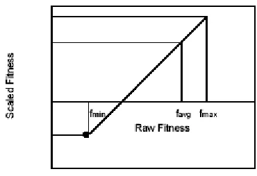
It is useful to scale the ‗raw‘ fitness scores to help avoid the above situations. This

algorithm uses linear scaling as described by Goldberg, Linear scaling produces a linear relationship between raw fitness, f, and scaled fitness, f’, as follows:

f’ = a f + b (1)

Coefficients a and b may be calculated as follows:

(2)

(3)

min

f f

f a

avg avg

m in *

m in

f f

f f

b

avg avg

Fig. 1. Linear Fitness Scaling

This scaling works fine for most situations, however in the later stages of evolution when

there are relatively few ‗low‘ scoring strategies problems may arise. The average and best

scoring strategies have very close raw fitness and extreme scaling is required to separate them. Applying this scaling to the few low scorers may result in them becoming negative. [Fig. 2]

Fig. 2. Linear Fitness Scaling Negative Values

This can be overcome by adjusting the scaling coefficients to scale the weak strategies to zero and scale the other strategies as much as is possible. In the case of negative scaled fitness values the coefficients may be calculated as follows:

(4)

(5)

Genetic object and applied to all raw fitness scores (i.e. the IPD payoffs) before performing genetic algorithm selection.

4.4. Reproduction

Having selected two strategies from the populat ion the Genetic Algorithm proceeds to mate these two parents and produce their two children. This reproduction is a mirror of sexual reproduction in which the genetic material of the parents is combined to produce the children. In this research reproduction allows exploration of the search space and provides a means of reaching new and hopefully better strategies. Reproduction is accomplished using two simple yet effective genetic operators–crossover and mutation.

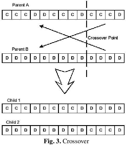
Crossover is an artificial implementation of the exchange of genetic information that occurs in real-life reproduction. This algorithm, breaking both the parent chromosomes at the same randomly chosen point and then rejoining the parts, can implement it. [Fig. 3]

Fig. 3. Crossover

This crossover action, when applied to strategies selected proportional to their fitness, constructs new ideas from high scoring building blocks. The genetic algorithm implemented in this research performs crossover a large percentage of the time, however occasionally (5% of the time by default) crossover will not be performed and simple natural selection will occur. In nature small mutations of the genetic material exchanged during reproduction occurs a very small percentage of the time. However if these

default) a bit copied between the parent and the child will be flipped, representing a mutation. These mutations provide a means of exploration to the search.

4.5. Replacement

The genetic algorithm is run across the population until it has produced enough children to build a new generation. The children then replace all of the original population. More complicated replacement techniques such as fit-weak and child parent replaced were researched but they were unsuitable for the round robin tournament nature of the system.

4.6. Search Termination

The only termination criteria implemented is a limit to the maximum number of generations that will run; the user may set this. Other termination criteria were investigated, for example detecting when a population has converged and strategies are receiving equal payoffs, however these criteria resulted in many false positives and it was decided better to allow the user to judge when the algorithm had reached the end of useful evolution.

5. Conclusion

GA often found strategies that scored substantially higher than any other algorithm. But it

would be wrong to conclude that the GA discovered strategies that are ―batter‖ than any

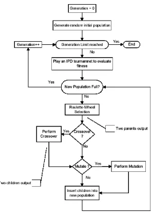
Appendix:

The following flowchart describes the completed genetic algorithm of the

Prisoner‘s Dilemma Problem.

References:

Axe lrod R, (1990). The Evolution of Cooperation, Penguin Books

B. Routledge, (1993). Co-Evolution and Spatia l Interaction, mimeo, Un iversity of British Colu mb ia

Cha mbers (ed.), (1995). Pract ical Handbook of Genetic A lgorith ms Applications, Volu me II, CRC Press

Conor Ryan, Niche Species, (1995). Formation in Genetic A lgorith ms, In L. Cha mbers (ed.), Practica l Handbook of Genetic A lgorith ms Applications Vo lu me I, CRC Press

David E. Go ldberg, (1989). Genetic Algorith ms in search, optimization, and machine learn ing, Addison-Wesley Publishing

Frank Schwe it zer, La xmidhar Behera, He in z Mühlenbein, (2002). Evolution of Cooperation in a Spatial Prisoner's Dile mma , Advances in Co mple x Systems, vol. 5, no. 2-3, pp. 269-299 John R. Koza, (1992). Genet ic Progra mming On the programming of computers by means of

natural selection, MIT Press

Peter J.B. Hancock, (1995). Se lection Methods for Evolutionary Algorith ms, In L. Geoff Bart lett, Genie : A First GA, In L. Chambe rs (ed.), Practica l Handbook of Genetic Algorith ms Applications, Vo lu me I, CRC Press

Shaun P. Hargreaves Heap and Yanis Varoufa kis, (1995). Ga me Theory a Crit ical Introduction, McGraw Hill Press