Geography, population density, and per capita income gaps across US states and Canadian provinces

Munich Personal RePEc Archive

Geography, population density, and

per-capita income gaps across US states

and Canadian provinces

Lagerlöf, Nils-Petter and Basher, Syed A.

October 2005

Online at

https://mpra.ub.uni-muenchen.de/369/

Geography, population density, and per-capita

income gaps across US states and Canadian

provinces

∗

Syed A. Basher

and Nils-Petter Lagerl¨of

Department of Economics, York University, Canada

September 28, 2006

∗_{We are grateful for comments from Tasso Adamopoulos, Ahmet Akyol, David}

An-dolfatto, Berta Esteve-Volart, Paul Klein, Shannon Seitz, and Andrei Semenov. Lagerl¨of thanks SSHRC for financial support. We also thank the following persons for help in lo-cating data sources: Katie Davis, ´Elise Laplaine and Greg LeBlanc of Statistics Canada; Karen D. Thompson of the US Census Bureau; Brian Dahlin and Serah Hyde of the Bureau of Labor Statistics; David Sutherland of NOAA; and Wendell Cox of Demographia.

†_{E-mail: basher@econ.yorku.ca.}

1

Introduction

This paper examines a novel link from geography to the distribution of per-capita incomes across US states and Canadian provinces. The existing liter-ature has often pointed to direct effects of geography, in particular vicinity to waterways and so-called natural harbors, to economic and demographic outcomes. Coastal regions are richer and more populated because they have more trading ports, goes the argument (see, in particular, Rappaport and Sachs 2003).

This explanation fails to account for why the Eastern half of North Amer-ica is richer and more densely populated than the Western half. It also fails to explain differences in population and per-capita incomes along the At-lantic coast: the US South and AtAt-lantic Canada are relatively poor, and New England is rich.

We believe there is something more involved than just a direct effect from geography. The way we think about these patterns relates to recent work explaining per-capita income gaps across countries through a chain of causation running from geography, via institutions, to current economic out-comes.1

The econometric approach taken in this literature is to use variables measuring geography and/or demography — such as settler mortality and pre-colonial population density — as exogenous instruments for some measure of institutions, for example an index over protection of property rights.

Using similar econometric techniques we document a related causal chain within the “neo-European” region of the USA and Canada. This chain runs from geography, via early settlement, population density, and education, to economic outcomes today. To see the point, note that five of the the six richest US states — Massachusetts, Connecticut, New York, New Jersey, and Delaware (see Table 1) — lie clustered in a belt along the Atlantic Ocean. This region was the first to be settled and from the start it has had the highest

1

population densities in North America. Here lie some of the world’s largest cities, like New York City and Boston, and highest ranked universities, such as Harvard, MIT, Yale, Cornell, and Princeton.2

Surrounding states and provinces have both sparser populations and lower per-capita incomes. (The reader may note that states to the south were all slave states; we return to this below.)

We propose that these patterns are due to geographical fundamentals which made the first Europeans settle in Northeastern USA: along the At-lantic coast, and where the climate was neither too hot (like in the US South), nor too cold (like in Canada). Early settlement has determined population densities and the location of urban centers up to this day, in turn affecting per-capita incomes, because such dense and urban environments are con-ducive to skill accumulation. This is also why so many top-ranked universi-ties lie in this region.

We combine PPP adjusted per-capita income data across 50 US states and 10 Canadian provinces, with measures of geography (such as average annual temperature, precipitation, and coastal dummies); population densities in 1900 and today; the sex ratio in 19003

; urbanization rates today; and the fraction of the population with a university degree today.

We first run a number of ordinary least-squares regressions showing that university education has a robust positive effect on per-capita incomes. It stays significant when controlling for political variables (such as the size of government and unionization); sectoral composition (like fisheries employ-ment); and a Canada dummy.

We then run a number of two-stage least squares regressions where

univer-2

One could add to this cluster Rhode Island, which is also densely populated and has an Ivy League university (Brown). However, it is not as rich as the other five (see Table 1). Interestingly, in 1840 Rhode Island was the richest state in the union, followed by those otherfive states; see Easterlin (1960, Table A-1). Why Rhode Island fell behind is a topic left for another paper.

3

sity education is instrumented with historical variables (population density in 1900, the sex ratio in 1900, and slavery in 1850). Wefind that these histor-ical variables are good instruments for university education, in the sense that they are highly correlated with university education and uncorrelated with the second-stage residual. That is, they seem to affect per-capita incomes through education, rather than directly.

The same conclusion holds when running other instrumental-variable re-gressions treating population density, the sex ratio, urbanization rates, and university education as endogenous. These are instrumented with various sets of geography variables, such as temperature, rainfall and coastal dummies. Again wefind that the instruments are valid: these geography variables seem to affect economic outcomes not directly but rather through their influence on, for example, population density and education.

In short, our results suggest that those five Northeastern states are so rich and densely populated because they lie by the Atlantic coast and have a climate which was inviting to settlers: neither too hot, nor too cold. For the same reason, their too hot, too cold, and too inland neighboring states and provinces are relatively poor and empty today.

We believe the value-added of this exercise is four-fold. First, as ar-gued already, our methodology relates closely to a new empirical develop-ment literature on geography, institutions, and income gaps. However, we seem to be the first to think about variation in per-capita incomes within a rich and “Neo-European” region, such as the US and Canada, using a sim-ilar instrumental-variable approach as, for example, Acemoglu et al. (2001, 2002).4

Second, we propose and test a link from geography to economic outcomes

4

which has been largely ignored in the existing literature: demographic and educational variables. This contrasts with e.g. Rappaport and Sachs (2003) who suggest that geography exerts a direct effect on economic outcomes across US regions, for example by affecting trade. It also contrasts with Acemoglu et al. (2001, 2002), and many others, who emphasize institutions (such as property rights) as the intermediate factor between geography and economic outcomes. Within the region we study institutions cannot (other than in a very broad sense) be the only factor involved, since much of the variation in per-capita incomes shows up across institutionally similar states and provinces (like New England and Atlantic Canada). Much of the causal-ity rather seems to run through the rise of urban centers, and the effect these have had on learning and human-capital accumulation.5

This is also consistent with a vast literature finding that shorter geographical distances facilitate skill accumulation (as discussed in Section 2.3).

Third, we do look at one particular institutional link from geography to economic outcomes: slavery. This institution arose in those regions of the Americas where the climate was suitable to grow staple crops like cotton, tobacco, and sugar: that is, in the Caribbean, Brazil, and the US South.6

Slavery has had well-documented negative effects on institutions (in the sense of, for instance, voting rights and school reforms), on equality, and on per-capita incomes today. This holds in our data too. More interestingly, how-ever, not only does slavery have a significantly negative effect on per-capita incomes in our regressions; including a slavery variable strengthens the ef-fect from population density. In some regressions the effect from population

5

In a sense, one could argue that our story partly mirrors the growth of Europe’s Atlantic regions following the discovery of the Americas (cf Acemoglu et al. 2005). It also relates to Glaeser et al. (2004) who think that European settlers brought not (only) their institutions, but (also) their human capital, although we suggest that population density and urbanization can by itself be a factor behind human capital accumulation and the rise of universities.

6

density is significantonly when we control for slavery. The intuition is that many former slave states are poorer today than their population densities alone would account for. Slavery picks up some of the variation in incomes, thereby also making the population density effect stronger. In that sense, the population-density link and the institutional link seem complimentary.

Fourth, we may add insights to a literature on differences in incomes and other variables across OECD countries, in particular between European countries and the US (Alesina et al. 2001, Gordon 2004, Prescott 2004, Rogerson 2005). Our methodology is a little different: we do not focus on labor supply or taxes; we run regressions rather than calibrating models; and (to iterate) we are the first to look at variation within the US-Canada region. However, our results may be interesting in light of this literature because Canada shares so many characteristics with both Europe and the US. (We return to this discussion in the conclusions in Section 4.)

The rest of this paper is organized as follows. Next Section 2 elaborates on the theory we wish to put forward and discusses how it seems to fit with the data. Section 3 presents the results, first when regressing per-capita incomes on university education and a number of control variables using ordinary least-squares, and then using various instrumental-variable approaches. Section 4 ends with a concluding discussion.

2

The theory and some preliminary evidence

The hypothesis that we are about to investigate can be summarized in aflow chart, as follows:

Geography _⇒ early settlement

⇒population density in 1900

⇒ population density today _⇒ accumulation of skills

⇒ per-capita income levels.

2.1

Geography and population density in 1900

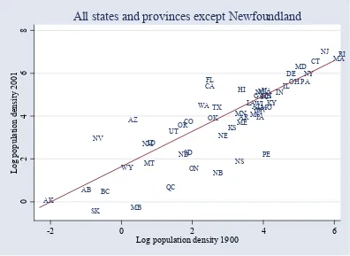
The first link runs from geography to early settlement. The earliest year for which we have population density data for most states and provinces is around 1900 (only data for Newfoundland is missing). Consider Figure 1 which plots average annual temperature against log population density in 1900. Consistent with Rappaport and Sachs (2003) it can be seen that Atlantic and other coastal states and provinces have higher densities than those located inland, at any given temperature (see Table 1 for a list of codes for all states and provinces). It also seems that the relationship between temperature and population density is ∩-shaped; very hot and very cold states and provinces are less densely populated than those at intermediate temperatures.

This ∩-shaped relationship is even more striking when looking only at the Atlantic region which is relatively homogenous in terms of, for example, mountainousness and rainfall (see Figure 2). As described in the introduc-tion, densities are high in a couple of Northeastern states and lower both to the north and the south of these. Note that there is nothing special about Canada, aside from the weather: in Figure 2 the fitted curve for US states only (dashed) is virtually identical to thefitted curve for states and provinces together (solid). Temperature thus accounts for Canada’s sparse population. Why does temperature have a non-monotonic effect on settlement? It makes sense that early settlers in North America, who were mostly farmers, avoided too cold regions due to their lower agricultural productivity.7

(The exception may be regions where they could procure food from fishing.) Hot regions may have been unsuitable for European settlers in particular, since they were not resistent to warm-weather diseases (Acemoglu et al. 2001; Coelho and McGuire 1997, 1999). Moreover, much of the migration to the warmer parts of the US were not by free Europeans but by African slaves,

7

without whom population density in the South would have been even lower. As discussed below, geography also seems to have had an effect on incomes through slavery, separate from the population density link.

Other geography variables which seem to have mattered is the number of rainy days per year (Figure 3) and total precipitation (Figure 4). These probably affected agricultural productivity.

All coasts, not only the Atlantic, have higher population densities than inland regions, and so do states and provinces around the Great Lakes. How-ever, the Atlantic is more densely populated than both the Gulf and Pacific coasts (see, for example, Map 2 in Rappaport and Sachs 2003; in fact, the whole eastern half of the US is more densely populated than the western half). The most probable explanation is that the Atlantic is closer to Europe, which is where most early settlers arrived from. Many immigrants stayed in the big cities where their ships landed. Trans-Atlantic trade may also have had an impact on early growth of the Atlantic region of North America, as it did on the European side of the Atlantic (Acemoglu et al. 2005).

2.2

Population density in 1900 and today

2.3

Population density and education

The idea that a shorter geographical distance between people enhances the exchange of ideas and accumulation of skills goes back at least to Jacobs (1969), and probably much longer (Glaeser 1999 quotes Alfred Marshall on agglomeration effects). Empirical support can be found in, for example, Jaffe et al. (1993), who show that patent citations are negatively related to distance. Glaeser and Mar´e (2001) find that wages are higher in cities because cities promote learning rather than the reverse causality by which skilled people choose to live in cities. Theoretical foundations can be found in, for example, Glaeser (1999).

It is also possible that colleges and universities, due to scale effects in education, have come to be located in regions with dense populations, both historically and today. Many Ivy League universities lie in the densely pop-ulated region around Northeastern USA, and vicinity to educational insti-tutions seems to matter for educational choice: Card (1995) finds that men who grew up near a four-year college have higher education and earnings, also when controlling for regional factors and family background; Glaeser and Saiz (2003) find that cities of a given size grow faster if they have more colleges per capita. A skilled labor force can also attract high-technology industries (Henderson et al. 1995).

2.3.1 Urbanization

Obviously, population per unit of land area over a whole state or province may not be the best measure of the mechanism we try to capture. Ideally one would want a measure of how well “connected” people are to the type of social networks which build skills and/or enhance growth of high-skilled industries. Alternatively one may want data over how far the average resident of a state or province is from the closest university or college.

measure we use is the fraction of the population living in cities exceeding the modest size of 1,000 people (we use this measure because it is the most comparable between Canada and the US). The fraction living in larger cities could perhaps have provided a betterfit.8

Moreover, urbanization rates may not be exactly the right measure either: population density may just as well serve as a proxy for whatever is the “true” measure.

These issues aside, we note that the signs are right: both log popula-tion density in 2001 and our measure of urbanizapopula-tion rates are positively correlated with the fraction of the population having a university degree (ur-banization slightly less than population density; see Table 2 and Figures 7 and 8).

2.3.2 The sex ratio in 1900

We do not have historical urbanization data (at least not for both Canada and the US) but a good proxy could be the sex ratio, that is, the number of men per woman. Edlund (2005) documents that rural areas in the Western world are relatively short on women, compared to urban areas. This seems particularly true in new settlements in colonial times. Guttentag and Secord (1983, Ch. 5) document that in frontier societies of the US men vastly outnumbered women into the 20th century, while the situation was rather the opposite in New England. (See also Angrist 2002.) This fits with our data, where the sex ratio in 1900 is strongly negatively correlated with log population density (Figure 11).

2.4

Education and per-capita incomes

The fraction with a university degree is highly positively correlated with per-capita incomes, notably more so than are population density in 2001

8

and urbanization (see Table 2). This suggests that the link from population density and urbanization to per-capita incomes does work through human capital.

2.5

Slavery

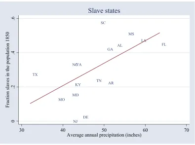
As seen in Figures 14 and 15 the fraction slaves in the population in 1850 varies with geographical variables, such as temperature and rainfall, which facilitated the growth of staple crops (see the discussion in the introduction). Slavery also seems to impact per-capita incomes and education today. The link is there when considering all states and provinces (Figure 16), and (more visibly) among slave states (Figures 17 and 18). Slavery thus constitutes a link from geography to economic outcomes, which does not work through population density.

3

Regression results

3.1

Ordinary least-squares regressions

Table 3 presents the ordinary least-squares results when regressing log per-capita income (GSP or GPP) on the fraction having a university degree and a number of other variables. University education has a high explanatory power on its own [an R-squared of 52.3% in column (1)]. It also stays very significant when controlling for a range of other control variables.

In all specifications but the first we enter a Canada dummy, which is mostly insignificant. One may note that it is consistently positive: when controlling for levels of university education (and a number of other variables) Canada does not seem to be poorer than the US, but rather richer. However, the Canada dummy tends to have a negative sign in the second stage of some of the instrumental-variable regressions shown later.

government, discriminatory taxation, and union density come out as signifi -cant (union density barely). These variables, however, are hard to interpret. They are all 1-10 indices, and it is not even always clear what a high or low score means (see Section A.3.6 in the appendix). Moreover, even though the sources do describe some of the details about how the FI variables are com-puted, the raw data is not provided and we have not been able to replicate these indices.

There is another problem with the FI variables. We computed an al-ternative set of political variables, with a clearer interpretation: the ratio of federal, state, and local government expenditure to incomes. As seen in column (10) of Table 3, a high ratio of federal expenditure to income has a significantly negative effect on per-capita income. But the direction of causal-ity is far from obvious. Notably, this variable is the highest and lowest for two Canadian provinces: Prince Edward Island (which is the poorest of all 60 states and provinces), and Alberta (the richest Canadian province). This probably reflects the Canadian federal government’s choices in response to existing income gaps, rather than exogenous causes behind the gaps. In other words, Ottawa does notmake Albertans rich by not giving them money; they

are rich and thus do not get any money.

The state and local spending ratios, on the other hand, are more plausible causes of per-capita income differences. However, as seen in column (11) and (12) these are insignificant, and of the “wrong” sign, respectively (that is, a bigger local government is associated with higher per-capita incomes).

Moreover, out of the three ratios the federal one is the most strongly correlated with FI’s size-of-government variable (the correlation coefficient is

−0.83). This is not strange because the FI variable is based on similar data. However, it does suggest that the size of government as measured by the Fraser Institute shows up as significant in these regressions, not because it causes income gaps, but rather because it is caused by existing gaps through federal expenditure.

or province’s labor force. The employment share in fisheries has a negative, but statistically insignificant, effect on per-capita incomes [column (14)]; the employment share in natural resources industries (mostly oil and gas) has a positive and significant effect [column (15)]. See also Figures 12 and 13.

However, data over fishery employment is available for only 33 states and provinces, and natural resource employment for 55 states and provinces. Most of the variation is among a few states and provinces, like Alaska, Al-berta, and Atlantic Canada (cf Figures 12 and 13). Endogeneity is also an issue. Canada’s Atlantic provinces may have come to rely more on fishery today because when fishery began its decline the labor force did not move into other sectors. Whatever prevented the growth of non-fishery industries should be the ultimate cause of current income gaps; we believe that cause is population density and education.

To sum up, the results shown in Table 3 suggest that university educa-tion has a robust positive and significant relationship with per-capita income levels. However, it is not clear whether education causes these income gaps, or if the causality goes the other way around. To address that issue we next turn to instrumental-variable analysis.

3.2

Two-stage least squares regressions

3.2.1 Historical variables as instruments

impact on education (cf Figure 18). The ultimate reason should be that slaves were often forbidden (or otherwise prevented) from learning to read or write. Also after abolition these effects seem to have lingered on. School reforms have tended to come later in formerly slave-dependent Caribbean countries and Brazil compared to Canada and the US north of the Chesapeake Bay (Mariscal and Sokoloff 2002), and there are indications of similar patterns within the US South (Lagerl¨of 2005).

Using measures from 1850 and 1900, rather than today, could also help alleviate some reverse-causality concerns: for example, high levels of educa-tion (and income) today may spur migraeduca-tion to cities today, but populaeduca-tion density a century back seems more likely to causally impact education today, rather than the other way around. (However, there are some caveats to this reasoning, as discussed below.)

The two-stage least squares results in Table 4 show that per-capita income is affected positively by the fraction with a university degree. This holds when this fraction is instrumented with the slavery variable, together with either log population density [column (1)], or the sex ratio [column (2)], as well as when using all three variables as instruments [column (3)].

To be valid instruments these variables shouldfirst of all be highly corre-lated with the instrumented variable. As seen in the lower panel of Table 4, the first-stage regressions do not have a very high R-squared (about 15%). However, anF-test shows that the instruments are jointly significant. More-over, although thefirst-stage estimated coefficients on log population density and the sex ratio are insignificant, their signs are the expected ones. That is, log population density has a positive effect on education, whereas slav-ery and the sex ratio have negative effects. However, the sex ratio gets the wrong sign when entered jointly with log population density since these two variables are highly correlated.

in-struments should be uncorrelated with the error terms in the second-stage regression. This seems to be the case: Hansen’s J-test does not reject the hypothesis that the second-stage error terms are uncorrelated with the in-struments; that is, the p-value is very high (well above conventional risk levels of 5% or 10%). To see that the instruments do not exert any direct impact on per-capita incomes we also report the results when letting each instrument enter the second-stage regression [columns (4) to (6)]. As seen, they all come out as insignificant.

All in all, it seems that these historical variables are valid instruments. However, in order to truly believe that they are valid we must also believe that the direction of causality runs from the instruments (population den-sity, the sex ratio, and slavery) to the instrumented variable (the fraction with university degree). The fact that the instruments date a century, or longer, back in time is no guarantee that this is the case. For example, some third factor may have made some states and provinces rich and highly edu-cated, and thus induced migrants to settle there, and thereby also made the economy less dependent on slave labor. In principle, what regions become prosperous and densely populated may be due to chance, and work through the coordination of many agents’ simultaneous decisions. However, we have already argued that there is one fundamental determinant of settlement in North America: geography.

3.2.2 Geography as instruments

instrumented. Generally, the results depend on how these choices are made: some instruments do a better job together with some endogenous (instru-mented) variables; other combinations do not work equally well.

A smaller set of geography instruments Table 5 shows the results

from a couple of two-stage least squares regressions where as instruments we use annual temperature and its square, and an Atlantic dummy (cf Figures 1 and 2). These are used to instrument log population density in 1900 or 2001, or the sex ratio in 1900. The dependent variable is log per-capita income.

As seen from the odd-numbered columns [(1), (3), and (5)], the results seem discouraging atfirst: for none of the three instrumented variables is the coefficient in the second-stage regression significant at any conventional risk level.

However, we recall from Figures 14 to 18 and the results in Table 4 that geography affects education and per-capita income also through slavery. We thus allow the fraction slaves in 1850 to enter the regression as an endogenous variable [columns (2), (4), and (6)]. As seen, not only does slavery come out as significant — the other three instrumented variables do too (at least at the 10% level), and they are also larger in size.

capital rather than institutions. So, in our data, does geography affect per-capita incomes through population density or through institutions? The answer is: both. It is not a matter of either/or; in fact, the effect from population density is seen only when controlling for institutions (that is, slavery).9

To understand why consider the plot of per-capita incomes and log popu-lation density in 2001 in Figure 9. As seen, those states which had the highest fraction slaves — Mississippi, South Carolina, and Louisiana — are outliers. They are thus poorer than their population densities can account for. When entering slavery into the regressions it picks up some of that variation in incomes, in effect making the population density effect stronger.

It is also interesting to note from the even-numbered columns in Table 5 that the Canada dummy comes out as significant in thefirst-stage regression but not in the second-stage regression when the instrumented variable is log population density in 2001; and vice versa when the instrumented variable is historical: either log population density in 1900 or the sex ratio in 1900. That is, there was nothing special about Canada by 1900: the sex ratios and population densities of Canadian provinces can be explained by geography. However, there is a negative “Canada effect” working after 1900 both on contemporary per-capita incomes and population densities.

The even-numbered columns of Table 5 also show that the instruments are good, in the sense that they perform well by Hansen’s overidentification test: zero correlation between the instruments and the second-stage residuals cannot be rejected based on the J-test, with p-values around 23-28%. The instruments are also jointly significant in the first-stage regression, as seen from the F-test in the lower panel (although the temperature variables do a poor job for the sex ratio).

9

A larger set of geography instruments Not only temperature and vicinity to the Atlantic have had an impact on population density. In Table 6 we use a larger set of geography variables as instruments. These are: average temperature and its square, average precipitation, average number of rainy days, and coastal dummies: for the Atlantic only in odd-numbered columns; and for the Atlantic and the Great Lakes in even-numbered.

We now use as endogenous (instrumented) variables log population den-sity in 1900 and 2001, as well as two variables through which these have supposedly affected per-capita incomes: urbanization rates, and university education. Slavery is also treated as endogenous and instrumented with the same variables (we do not report the first-stage regression).

Again, as seen in Table 6, wefind that the instrumented variables overall have a significant effect on per-capita incomes, most withp-values below 5%. When we instrument urbanization rates the effect is insignificant when using the Atlantic dummy only [column (5)], but becomes significant at the 10% level when adding the Great Lakes dummy [column (6)].

The instruments seem to be valid too. The F-test in the first-stage re-gression suggests the instruments are jointly significant (even though many of the instruments are individually highly insignificant). Also, Hansen’s J-test for overidentification suggests that the instruments are uncorrelated with the residuals in the second-stage regression.

We may also note that slavery comes out as insignificant when university education is instrumented but not when population density is instrumented. This suggests that the negative effect from slavery to economic outcomes works through education. This is consistent with, for example, Mariscal and Sokoloff (2000) and Lagerl¨of (2005).

4

Discussion and concluding remarks

Ed-ward Island was the poorest with a per-capita Gross Province Product of US$20,545. Their per-capita income ratio was thus about 2.25. This paper is about explaining such income gaps.

One may argue that this is not an interesting research topic: 2.25 is not a huge gap by international standards; across countries per-capita income gaps can exceed a factor of 30 or 40. One reason that we still find this topic interesting is that different North American regions share a lot (though not everything) in geography, history, institutions, language, and ethnicity. Comparing income gaps across states and provinces of North America thus amounts to keeping such factors constant, to some extent, and this can teach us a great deal also about cross-country income gaps.

Our explanation builds around a chain of causation. Geography mat-tered for where Europeans settled which determined where cities and urban centers are located today. This has impacted per-capita income patterns be-cause cities are conducive to skill accumulation. We test this hypothesis with various instrumental variable specifications and the data does not reject it.

Population density may play some role for cross-country income gaps too: it usually shows up with a positive sign in per-capita income regressions (Olson 1996), and city-states like Luxembourg, Hong Kong, and Singapore are rich. However, it seems plausible that in a world-wide context geography may exert a much stronger effect through institutions; in the region we study the population-density effect shows up more clearly because the US and Canada have so similar institutions.

Some would suggest other explanations than those we propose. Within the US-Canada region the poorest locations lie in Atlantic Canada (Table 1). It may thus be tempting to attribute income gaps across this region to variations in the dependence on fishery. But this is not an exhaustive explanation, we argue. There are other poor regions which do not rely on

have any significant fishery industries, and our regression results are not too supportive of a fishery explanation (see Section 3 and Figure 13).

Moreover, it is not obvious why the decline of one sector of the economy would necessarily mean the decline of a whole region. If fishery has declined, why have people previously employed in the fisheries not moved to other sectors? Consider Massachusetts, a maritime region which once had afishery and whaling industry, and is rich today and not dependent onfishery. What makes Nova Scotia different from Massachusetts? Why could not Halifax be like Boston? A good explanation should be deeper than simply pointing to the decline of some sector of the economy. It should point to fundamental causes (like geography), rather than proximate.

Our results are also interesting when thinking about income gaps between European countries, US states, and Canadian provinces. The fact that the richest regions of the United States are the most densely populated suggests that per-capita income gaps between Europe and the US cannot be explained by the same factor, since most European countries are poorer and more densely populated than the US. Some would explain Europe’s relative poverty by emphasizing that the US has a smaller government, lower taxes, and a less regulated labor market. In the US-Canada case such explanations have been put forward by the Fraser Institute. We do not rule such explanations out but here they do not seem to tell the whole story. For example, we find that while government expenditure (relative to income) is negatively correlated with per-capita income, the correlation holds only for federal expenditures but not for state and local. The causation thus seems to go from poverty to spending, rather than the other way around. That is, poor regions receive more transfers from benevolent politicians in Ottawa and Washington.

A

Data appendix

Below we list our data sources, some of which are available online only. When it is not self-explanatory we try to describe in as much detail as possible what steps to take to access the online data. All data are also available as a STATA

file at:

http://www.arts.yorku.ca/econ/lagerloef/HP/PubDataUSCan.dta

A.1

Geography variables

A.1.1 Temperature, precipitation, and rainy days

Data for three weather variables were retrieved from the Weatherbase Web site at www.weatherbase.com. These are: average temperature over the year (in degrees Fahrenheit); average precipitation (inches of rainfall over the year); and average number of rainy days per year.

Where available these refer to the capital of the state or province (see Table 1 for a list). Else another city was chosen alphabetically. For tem-perature and precipitation, data from Nova Scotia refer to Ecum Secum; all other temperature and precipitation data refer to the capital.

Rainy days data for capitals were often missing, in which case we used data for these cities: Banff, Alberta; Abbotsford, British Columbia; Brandon, Manitoba; Belle Isle, Newfoundland; Ecum Secum, Nova Scotia; Armstrong, Ontario; Alma, Quebec; Bowling Green, Kentucky; Aberdeen, Maryland; Alexandria, Minnesota; Belton, Missouri; Battle Mountain, Nevada; Atlantic City, New Jersey. For all other states and provinces we used the capital.

A.1.2 Coastal dummies

Massachusetts, New Hampshire, New Jersey, New York, North Carolina, Rhode Island, South Carolina, and Virginia.10

The following states and provinces are considered to be located by the Great Lakes: Ontario, Illinois, Indiana, Michigan, Minnesota, New York, Ohio, Pennsylvania, and Wisconsin.

A.2

Historical variables

A.2.1 The fraction slaves in 1850

The fraction slaves in the population is calculated as the total number of slaves in 1850 over total population in 1850. This data is made available by the Geospatial and Statistical Data Center at the University of Virginia Library. Their Web site is at:

http://fisher.lib.virginia.edu/collections/stats/histcensus/

Canada did not use slavery.

A.2.2 The sex ratio in 1900

The numbers of males and females in Canada refer to the year 1901 and are from Census of Canada (1902, Table III).

The corresponding data for the US were extracted from the Geospatial and Statistical Data Center, University of Virginia Library (see the previous section; click on 1900 and follow the links).

Note that the Canadian data is for 1901 and the US data is for 1900, but we refer to this variable as the sex ratio in 1900.

10

A.2.3 Population density in 1900

The Canadian population density data are from Series A54-66: Population density per square mile, Canada and provinces, 1871 to 1976, Statistics Canada (1983).

US population density is from Table 5, Statistical abstract of the United States 1901, which is available at

http://www.census.gov/statab/www/

Note that the Canadian data is for 1901 and the US data is for 1900, but we refer to this variable as population density in 1900.

A.3

Contemporary variables

A.3.1 GDP per capita

PPP adjusted GDP per capita for both Canadian provinces and US states are from the Web site Demographia run by the Wendell Cox Consultancy, at www.demographia.com. All figures are for 1999 and in current US dollars. The exact links are:

http://www.demographia.com/db-cangdpr99.htm (for Canada) http://www.demographia.com/db-usgdpr99.htm (for the US)

Note that the state and province level equivalents of GDP are called GSP (Gross State Product) and GPP (Gross Province Product), respectively. In the text we also call this variable per-capita income for short.

A.3.2 Fishery and natural resource data

Natural resource employment By employment in natural resource

http://data.bls.gov/PDQ/outside.jsp?survey=sm

For both Canada and the US the numbers are from 2000.

Fishery employment The number of people employed infisheries in Canada

are downloaded electronically from the Statistics Canada Web site, at www.statcan.ca. To access the data, select census; select data; select topic-based tabulations;

click on number 11 — “Canada’s workforce: paid work.” Table 8 provides the number of people employed by industry and province.

The US data are from Pritchard (2003, p. 95), under the category “em-ployment, craft, and plants.” The US data refer to total employment in both the fish-processing and wholesale industry.

For both Canada and the US these numbers are from 2001.

Total employment To get fishery and natural resource employment as

fractions of total employment we use the following data. For Canadian provinces, 2000 and 2001 total employment is from Statistics Canada (2003, Table 18), available online at www.statcan.ca.

For the US total employment in 2000 is from Table 572, Statistical Ab-stract of the United States 2001, US Census Bureau, available online at http://www.census.gov/statab/www/. Total employment for 2001 is from Table 565, Statistical Abstract of the United States 2002, also available on-line at http://www.census.gov/statab/www/.

A.3.3 Urbanization rates

For the US the corresponding numbers are from the US Census Bureau’s 2000 Summary File 1 (SF 1) 100-Percent data (Table P2), available online at http://factfinder.census.gov.

For both Canada and the US these numbers are from 2000.

A.3.4 Population density in 2001

Population density per square kilometer for Canadian provinces was down-loaded electronically from the Statistics Canada Web site, at www.statcan.ca, using the following steps: select learning resources; select E-STAT; select ta-ble of contents; select people; select data; select population and demography; from the census databases select population characteristics; select 2001 pop-ulation and dwelling counts; select the desired item from the list. One square mile is 2.59 square kilometers.

For US states population density per square mile is collected from Ta-ble 19, Statistical abstract of the United States 2002, US Census Bureau, available online at http://www.census.gov/statab/www/.

For both Canada and the US these numbers are from 2001.

A.3.5 Fraction with a university degree

For Canada this fraction is given by the number of persons 15 years and over with a university (Bachelor) degree, divided by total population 15 and over. The number of persons with a degree are from Statistics Canada, 2001 Census, downloaded electronically from the Statistics Canada Web site, www.statcan.ca, following these steps: select census; select search by topic; select education in Canada: school attendance and levels of schooling; click on number 1 (under topic-based tabulations) — detailed highest level of schooling. Total population numbers are from the same Web site: select census; select search by topic; select age and sex; click on number 2, “profile of age and sex.”

Table 231, Statistical Abstract of the United States 2003, US Census Bureau, available at http://www.census.gov/statab/www/.

The Canadian data is from 2001 and the US data from 2000.

A.3.6 Political variables

Fraser Institute indicators We use six political indicators constructed

by the Fraser Institute (FI), a Canadian think tank. These are meant to measure “economic freedom” and/or theflexibility of labor markets and take values on a scale from 1 to 10. Indicators A to D below are from Karabegovi´c et al. (2004); indicators E and F from Clemens et al. (2004).

Indicator A: “Size of the government” is an index measuring general gov-ernment consumption expenditures relative to GSP or GPP. A higher score means smaller government.

Indicator B: “Discriminatory taxation” is an index measuring how “dis-criminatory” the tax system is; taxation is considered discriminatory if, for instance, the link between taxes paid and services received is weak, or marginal taxes are high. A higher score means less discriminatory taxation.

Indicator C: “Minimum wage legislation” is an index measuring the an-nual income earned by someone working at the minimum wage relative to per-capita GSP or GPP. A higher score means a higher minimum wage.

Indicator D: “Union density” is an index measuring the fraction of the work force who is unionized. A higher score means that a larger fraction is unionized.

Indicator E: “Average duration of unemployment” is an index measuring just that. A higher score means longer unemployment duration.

Indicator F: “Flexibility in labor-relation laws” is an index measuring the

flexibility in different areas of labor law. A higher score means that labor laws are more flexible.

Government expenditure Aside from the variables from the Fraser

state/provincial, and local government expenditure to income.

Data over government expenditures across Canadian provinces are from Statistics Canada (2003, Table 7-9). We first divided expenditure by popu-lation to get it in per-capita terms; we then divided by per-capita personal income to get the total expenditure as a fraction of income. Both population and per-capita personal income by province were collected from Statistics Canada (2003, Table 18).

The same data for US states are from Sagoo (2005; Tables C18, E15, and F14). To get total expenditure as a fraction of income we divided per-capita expenditures by per-per-capita personal income (collected from Table A14 in Ibid.).

These sources are partly the same as those used to calculate FI’s index over the size of government (Indicator A above).

References

[1] Angrist, J., 2002, How do sex ratios affect marriage and labor mar-kets? Evidence from America’s second generation, Quarterly Journal of Economics 117, 997-1038.

[2] Acemoglu, D., S. Johnson, and J.A. Robinson, 2001, The colonial ori-gins of comparative development: an empirical investigation, American Economic Review 91, 1369-1402.

[3] − − −, 2002, Reversal of fortune: geography and institutions in the making of the modern world income distribution, Quarterly Journal of Economics 117, 1231-1294.

[4] − − −, 2005, The rise of Europe: Atlantic trade, institutional change and growth, American Economic Review, 95, 546-579.

[5] Alesina, A., E.G. Glaeser, and B. Sacerdote, 2001, Why doesn’t the US have a European-style welfare state?, mimeo, Harvard University.

[6] Banerjee, A., and L. Iyer, 2005, History, institutions, and economic per-formance: the legacy of colonial land tenure systems in India, American Economic Review 95, 1190-1213.

[7] Barro, R.J., and X. Sala-i-Martin, 1992, Convergence, Journal of Polit-ical Economy 100, 223-251.

[8] Berkowitz, D. and K. Clay, 2004, Initial conditions, institutional dynam-ics and economic performance: evidence from American states, mimeo, University of Pittsburgh.

[10] Census of Canada, 1902, Fourth census, volume 1: population, printed by S.E. Dawson, Ottawa.

[11] Clemens, J., K. Godin, A. Karabegovi´c, and N. Veldhuis, 2004, Measur-ing labour markets in Canada and the United States, Fraser Institute.

[12] Coelho, P.R.P., and R.A. McGuire, 1997, African and European bound labor in the New World: The biological consequences of economic choices, Journal of Economic History 57, 83-115.

[13] _{− − −}, 1999, Biology, diseases, and economics: an epidemiological his-tory of slavery in the American South. Journal of Bioeconomics 1, 151-190.

[14] Collard, I.F., and R.A. Foley, 2002, Latitudinal patterns and environ-mental determinants of recent human cultural diversity: do humans fol-low biogeographical rules?, Evolutionary Ecology Research 4, 371-383.

[15] Easterlin, R.A., 1960, Interregional differences in per capita income, population, and total income, 1840-1950, in: Trends in the American economy in the nineteenth century, Princeton University Press (for the NBER).

[16] Easterly, W. and R. Levine, 2003, Tropics, germs, and crops: the role of endowments in economic development, Journal of Monetary Economics, 50, 3-39.

[17] Edlund, L., 2005, Sex and the city, Scandinavian Journal of Economics 107, 25-44.

[18] Engerman, S.L., and K.L, Sokoloff, 2002, Factor endowments, inequality, and paths of development among New World economies, Economia 3, 41-109.

[20] Glaeser, E.L., 1999, Learning in cities, Journal of Urban Economics 46, 254-277.

[21] Glaeser, E.L., and D.C. Mar´e, 2001, Cities and skills, Journal of Labor Economics 19, 316-342.

[22] Glaeser, E.L., and A. Saiz, 2003, The rise and fall of the skilled city, mimeo, Harvard University.

[23] Glaeser, E.L., R. La Porta, F. Lopez-de-Silanes, and A. Shleifer, 2004, Do institutions cause growth?, Journal of Economic Growth 9, 271-303.

[24] Gordon, R., 2004, Two centuries of economic growth: Europe chasing the American frontier. mimeo, Northwestern University.

[25] Guttentag, M., and P.F. Secord, 1983, Too many women? The sex ratio question, Sage Publications, Beverly Hills, California.

[26] Henderson, V., A. Kuncoro, M. Turner, 1995, Industrial development in cities, Journal of Political Economy 103, 1067-1090.

[27] Jacobs, J., 1969, The economy of cities, Random House, New York.

[28] Jaffe, A.B., M. Trajtenberg, R. Henderson, 1993, Geographic localiza-tion of knowledge spillovers as evidenced by patent citalocaliza-tions, Quarterly Journal of Economics 108, 577-598.

[29] Karabegovi´c, A., F. McMahon, D. Samida, and G. Mitchell, 2004, Eco-nomic freedom of North America, annual report, Fraser Institute.

[30] Lagerl¨of, N.P., 2005, Geography, institutions, and growth: the United States as a microcosm, mimeo, York University.

policy, history, and political economy, Hoover Institution Press, Stan-ford, California.

[32] Mitchener, K.J., and I.W. McLean, 2003, The productivity of US states since 1880, Journal of Economic Growth 8, 73-114.

[33] Olson, M., 1996, Big bills left on the sidewalk: why some countries are rich, and others poor, Journal of Economic Perspectives 10, 3-24.

[34] Prescott, E.C., 2004, Why do Americans work so much more than Eu-ropeans?. Federal Reserve Bank of Minneapolis Quarterly Review 28, 2-13.

[35] Pritchard, E.S. (ed.), 2003, Fisheries of the United States 2002, Na-tional Marine Fisheries Services, NOAA, Silver Spring, Maryland, http://www.st.nmfs.gov/st1/fus/current/2002-fus.pdf

[36] Rappaport, J., 2004, Moving to nice weather, RWP 03-07 Federal Re-serve Bank of Kansas City.

[37] Rappaport, J., and J.D. Sachs, 2003, The United States as a coastal nation, Journal of Economic Growth 8, 5-46.

[38] Rodrik, D., A. Subramanian, and F. Trebbi, 2004, Institutions rule: the primacy of institutions over geography and integration in economic development, Journal of Economic Growth 9, 131-165.

[39] Rogerson, R., 2005, Structural transformation and the deterioration of European labor market outcomes, mimeo, Arizona State University.

[40] Sachs, J.D., 2001, Tropical underdevelopment, NBER working paper 8119.

[42] _{− − −}, 2003, Institutions don’t rule: direct effects of geography on per-capita income, NBER working paper 9490.

[43] Statistics Canada, 1983, Electronic edition of historical statis-tics of Canada, second edition, Catalogue no. 11-516-XIE, http://www.statcan.ca/english/freepub/11-516-XIE/sectiona/toc.htm

[44] _{− − −}, 2002, Human activity and the

environ-ment, Annual statistics, Catalogue No. 16-201-XIE,

http://estat.statcan.ca/content/english/articles/other/other-envi1.pdf

[45] ₋₋₋, 2003, Provincial Economic Accounts, Catalogue No. 13-213-PPB, http://www.statcan.ca:8096/bsolc/english/bsolc?catno=13-213-P

[46] Sokoloff, K.L., and S.L. Engerman, 2000, History lessons: Institutions, factor endowments, and paths of development in the New World, Journal of Economic Perspectives 14, 217-232.

AB BC MB NB NS ON PE QC SK AL AK AZ AR CA CO CT DE FL GA HI ID IL IN IA KS KY LA ME MD MA MI MN MS MO MT NE NV NH NJ NM NY NC ND OH OK OR PA RI SC SD TN TX UT VT VA WA WV WI WY -2 0 2 4 6 L og popul at ion de ns it y 1 900

30 40 50 60 70 80

Average annual temperature (Fahrenheit)

All states and provinces except Newfoundland.

Figure 1. Temperature and population density.

NB NS PE QC CT DE FL GA ME MD MA NH NJ NY NC RI SC VA 1 2 3 4 5 6 L og popul at ion de ns it y 1 900

40 50 60 70

Average annual temperature (Fahrenheit)

Atlantic states and provinces except Newfoundland.

AB BC MB NB NS ON PE QC SK AL AK AZ AR CA CO CT DE FL GA HI ID IL IN IA KS KY LA ME MD MA MI MN MS MO MT NE NV NH NJ NM NY NC ND OH OK OR PA RI SC SD TN TX UT VT VA WA WV WI WY -2 0 2 4 6 L og popul at ion de ns it y 1 900

0 50 100 150 200

Average number of rainy days per year

All states and provinces except Newfoundland

Figure 3: Population density and number of rainy days.

AB BC MB NB NS ON PE QC SK AL AK AZ AR CA CO CT DE FL GA HI ID IL IN IA KS KY LA ME MD MA MI MN MS MO MT NE NV NH NJ NM NY NC ND OH OK OR PA RI SC SD TN TX UT VT VA WA WV WI WY -2 0 2 4 6 L og popul at ion de ns it y 1 900

10 20 30 40 50 60

Average annual precipitation (inches)

AB _BC MB NB NS ON PE QC SK AL AK AZ AR CA CO CT DE FL GA HI ID IL IN IA KS KY LA ME MD MA MI

MN MSMO

MT NE NV NH NJ NM NY NC ND OH OK OR PA RI SC SD TN TX UT VT VA WA WV WI WY 0 2 4 6 8 L og popul at ion de ns it y 2 001

-2 0 2 4 6

Log population density 1900

All states and provinces except Newfoundland

Figure 5: Population density a century ago and today.

AB BC MB NB NL NS ON PE QC SK AL AK AZ AR CA CO CT DE FL GA HI ID IL IN IA KS KY LA ME MD MA MI MN MS MO MT NE NV NH NJ NM NY NC ND OH OK OR PA RI SC SD TN TX UT VT VA WA WV WI WY .4 .6 .8 1 U rba ni za ti on ra te

0 2 4 6 8

Log population density 2001

AB BC MB NB NL NS ON PE QC SK AL AK AZ AR CA CO CT DE FL GA HI ID IL IN IA KS KY LA ME MD MA MI MN MS MO MT NE NV NH NJ NM NY NC ND OH OK OR PA RI SC SD TN TX UT VT VA WA WV WI WY .1 .1 5 .2 .2 5 .3 .3 5 F ra ct ion w it h uni ve rs it y de gre e

.4 .6 .8 1

Urbanization rate

All states and provinces

Figure 7: Urbanization and university education.

AB BC MB NB NL NS ON PE QC SK AL AK AZ AR CA CO CT DE FL GA HI ID IL IN IA KS KY LA ME MD MA MI MN MS MO MT NE NV NH NJ NM NY NC ND OH OK OR PA RI SC SD TN TX UT VT VA WA WV WI WY .1 .1 5 .2 .2 5 .3 .3 5 F ra ct ion w it h uni ve rs it y de gre e

0 2 4 6 8

Log population density 2001

AB BC MB NB NL NS ON PE QC SK AL AK AZ AR CA CO CT DE FL GA HI ID IL IN IA KS KY LA ME MD MA MI MN MS MO MT NE NV NH NJ NM NY NC ND OH OK OR PA RI SC SD TN TX UT _VT VA WA WV WI WY 10 10. 2 10. 4 10. 6 10. 8 L og pe r-c ap it a G S P or G P P

0 2 4 6 8

Log population density 2001

All states and provinces

Figure 9: Population density and per-capita income.

AB BC MB NB NL NS ON PE QC SK AL AK AZ AR CA CO CT DE FL GA HI ID IL IN IA KS KY LA ME MD MA MI MN MS MO MT NE NV NH NJ NM NY NC ND OH OK OR PA RI SC SD TN TX UT _VT VA WA WV WI WY 10 10. 2 10. 4 10. 6 10. 8 L og pe r-c ap it a G S P or G P P

.1 .15 .2 .25 .3 .35

Fraction with university degree

BC MB NB NS ON PE QC AL AR CA CO CT DE FL GA ID IL IN IA KS KY LA ME MD MA MI MN MS MO MT NE NV

NH _NY NJ

NC ND OH OR PA RI SC SD TN TX UT _VT VA WA WV WI WY .8 1 1. 2 1. 4 1. 6 1. 8 S ex ra ti o (num be r of m en pe r w o m an) 1 900

-2 0 2 4 6

Log population density 1900

For 52 states and provinces where data was available

Figure 11: Sex ratio and population density a century ago.

AB BC MB NB NL NS ON

QCAL _SK

AK AZ AR CA CO CT FL GA ID IL IN IA KS KY LA ME MA MI MN MS MO MT NV NH NJ NM NY NC ND OH OK OR PA RI SC SD TN TX UT VT VA WA WV WI WY 10 10. 2 10. 4 10. 6 10. 8 L og pe r-c ap it a G S P or G P P

0 .02 .04 .06

Fraction working in natural resource industries

AB BC MB NB NL NS ON PE QC SKAL AK CA CT DE FL GA LA ME MD MA MS NH NJ NY NC OR PARI SC TXVA WA 10 10. 2 10. 4 10. 6 10. 8 L og pe r-c ap it a G S P or G P P

0 .02 .04 .06

Fraction working in fisheries

For 33 states and provinces where data was available

Figure 13: Employment in fisheries and per-capita income.

AL AR DE FL GA KY LA MD MS MO NJ NC SC TN TX VA 0 .2 .4 .6 F ra ct ion s la ve s i n t he popul at ion 1850

50 55 60 65 70

Average annual temperature (Fahrenheit)

AL AR DE FL GA KY LA MD MS MO NJ NC SC TN TX VA 0 .2 .4 .6 F ra ct ion s la ve s i n t he popul at ion 1850

30 40 50 60 70

Average annual precipitation (inches)

Slave states

Figure 15: Slavery and rainfall across slave states.

AB BC MB NB NL NS ON PE QC SK AL AK AZ AR CA CO CT DE FL GA HI ID IL IN IA KS KY LA ME MD MA MI MN MS MO MT NE NV NH NJ NM NY NC ND OH OK OR PA RI SC SD TN TX UT VT VA WA WV WI WY 10 10. 2 10. 4 10. 6 10. 8 L og pe r-c ap it a G S P or G P P

0 .2 .4 .6

Fraction slaves in the population 1850

AL AR DE FL GA KY LA MD MS MO NJ NC SC TN TX VA 10 10. 2 10. 4 10. 6 10. 8 L og pe r-c ap it a G S P or G P P

0 .2 .4 .6

Fraction slaves in the population 1850

Slave states

Figure 17: Slavery and per-capita income across slave states.

AL AR DE FL GA KY LA MD MS MO NJ NC SC TN TX VA .1 5 .2 .2 5 .3 .3 5 F ra ct ion w it h uni ve rs it y de gre e

0 .2 .4 .6

Fraction slaves in the population 1850

Slave states

State or Per-capita GSP or State or Per-capita GSP or

province or GPP (US$), 1999 province or GPP (US$), 1999

1 Connecticut CT Hartford 46,245 31 Tennessee TN Nashville 31,017 2 Delaware DE Dover 46,008 32 Indiana IN Indianapolis 30,659

3 Alaska AK Juneau 42,539 33 Kansas KS Topeka 30,460

4 Massachusetts MA Boston 42,519 34 Arizona AZ Phoenix 30,070

5 New York NY Albany 41,469 35 Iowa IA Des Moines 29,707

6 New Jersey NJ Trenton 40,713 36 South Dakota SD Pierre 29,505 7 Nevada NV Carson City 38,615 37 Louisiana LA Baton Rouge 29,496 8 Colorado CO Denver 37,900 38 Utah UT Salt Lake City 29,411 9 California CA Sacramento 37,082 39 New Mexico NM Santa Fe 29,328 10 New Hampshire NH Concord 36,823 40 Florida FL Tallahassee 29,309 11 Illinois IL Springfield 36,746 41 Vermont VT Montpelier 28,908 12 Wyoming WY Cheyenne 36,380 42 Kentucky KY Frankfort 28,665 13 Washington WA Olympia 36,352 43 South Carolina SC Columbia 27,515 14 Minnesota MN Saint Paul 36,223 44 Maine ME Augusta 27,185

15 Georgia GA Atlanta 35,402 45 Idaho ID Boise 27,183

16 Virginia VA Richmond 35,243 46 North Dakota ND Bismarck 26,814

17 Alberta AB Edmonton 34,540 47 Quebec QC Quebec City 26,432

18 Hawaii HI Honolulu 34,512 48 Alabama AL Montgomery 26,333 19 Texas TX Austin 34,288 49 Saskatchewan SK Regina 26,094 20 North Carolina NC Raleigh 33,799 50 British Columbia BC Victoria 26,086 21 Maryland MD Annapolis 33,782 51 Oklahoma OK Oklahoma City 25,724 22 Oregon OR Salem 33,079 52 Arkansas AR Little Rock 25,388 23 Rhode Island RI Providence 32,848 53 Manitoba MB Winnipeg 25,328

24 Ontario ON Toronto 32,373 54 Montana MT Helena 23,376

25 Nebraska NE Lincoln 32,259 55 Mississippi MS Jackson 23,220 26 Ohio OH Columbus 32,157 56 West Virginia WV Charleston 22,516 27 Pennsylvania PA Harrisburg 31,931 57 Nova Scotia NS Halifax 22,336 28 Wisconsin WI Madison 31,708 58 New Brunswick NB Fredericton 22,187 29 Michigan MI Lansing 31,257 59 Newfoundland NL St. John's 21,008 30 Missouri MO Jefferson City 31,174 60 Prince Edward Island PE Charlottetown 20,545

Rank Rank

Table 1: List of states/provinces and per-capita incomes

Capital Capital

Log per-capita Fraction with Urbanization Log population Log population GSP or GPP university degree rate density 2001 density 1900 Log per-capita GSP or GPP 1.000

Fraction with university degree 0.723 1.000

Urbanization rate 0.647 0.393 1.000

Log population density 2001 0.508 0.654 0.334 1.000

Log population density 1900 0.176 0.361 0.009 0.841 1.000

Table 2: Correlation matrix

(1) (2) (3) (4) (5) (6) (7) (8) 9.811 9.719 9.231 9.206 9.684 9.926 9.566 9.596 (0.000) (0.000) (0.000) (0.000) (0.000) (0.000) (0.000) (0.000)

Fraction with 2.297 2.642 1.661 2.311 2.627 2.456 2.716 2.709 university degree (0.000) (0.000) (0.000) (0.000) (0.000) (0.000) (0.000) (0.000)

0.074 0.128 0.207 0.055 0.012 0.164 0.112 (0.280) (0.016) (0.004) (0.457) (0.862) (0.252) (0.129)

0.100 (0.000)

Discriminatory 0.104 taxation (FI) ( 0.000)

Average unem- 0.003

ployment duration (FI) (0.483)

-0.022 (0.059)

Felixibility in 0.015

labor laws (FI) (0.474)

Minimum-wage 0.016

legislation (FI) (0.172)

(9) (10) (11) (12) (13) (14) (15) (16) 9.184 10.184 9.747 9.540 10.045 9.615 9.595 9.396 (0.000) (0.000) (0.000) (0.000) (0.000) (0.000) (0.000) (0.000)

Fraction with 1.347 1.898 2.573 2.698 1.997 3.193 3.015 3.894 university degree (0.000) (0.000) (0.000) (0.000) (0.000) (0.000) (0.000) (0.000)

0.032 0.032 0.062 0.147 0.094 0.145 0.124 0.210 (0.748) (0.580) (0.376) (0.060) (0.180) (0.125) (0.055) (0.004)

0.084 ( 0.000) Discriminatory 0.069

taxation (FI) ( 0.006) Average unem- 0.006 ployment duration (FI) ( 0.073)

-0.019 ( 0.038) Felixibility in -0.018 labor laws (FI) ( 0.392) Minimum-wage 0.008 legislation (FI) ( 0.329)

Ratio of federal -1.174 -1.212 expenditure to income ( 0.000) ( 0.000)

Ratio of state -0.021 0.026 expenditure to income ( 0.378) ( 0.240)

Ratio of local 1.416 0.944 expenditure to income ( 0.060) ( 0.160)

Fraction working -2.479 -2.530

in fisheries ( 0.156) ( 0.115)

Fraction working in na- 3.313 5.188 tural resource industries ( 0.027) ( 0.004)

R-squared 0.523 0.533 0.746 0.537 0.562 0.537 0.548 60

0.643 Union density (FI)

60

No. of observations 60

Constant

Canada dummy

60 60 60 Size of government (FI)

60 60

30

60 60 60 60

Union density (FI)

60 33 55

Panel B: specifications (9) to (16)

Table 3: Higher education and per-capita income: ordinary least-squares regressions Dependent variable is log per-capita GSP or GPP

Panel A: specifications (1) to (8)

No. of observations Constant

Canada dummy

(1) (2) (3) (4) (5) (6) 9.686 9.619 9.565 9.556 9.467 9.624 (0.000) (0.000) (0.000) (0.000) (0.000) (0.000)

Fraction with 2.776 3.046 3.265 3.314 3.411 3.038

university degree (0.000) (0.000) (0.001) (0.000) (0.000) (0.252)

0.100 0.081 0.106 0.109 0.120 0.077 (0.393) (0.483) ( 0.359) ( 0.260) ( 0.230) ( 0.819)

Log population -0.001

density 1900 ( 0.955)

0.055 ( 0.712)

Fraction slaves -0.029

in 1850 (0.913)

Hansen J statistic 0.393 0.114 0.595 0.553 0.377 0.596

Degrees of freedom 1 1 2 1 1 1

Chi-Sqr test (p-value) ( 0.530) (0.735) (0.742) (0.457) ( 0.539) (0.440)

0.244 0.314 (0.000) (0.000)

-0.114 -0.121 (0.000) (0.000) Log population 0.004

density 1900 ( 0.128)

-0.048 (0.133) Fraction slaves -0.091 -0.101

in 1850 (0.001) (0.001) Partial R-squared

of excluded instruments

F-statistic for joint significance of excl. instr.

F-test (p-value) (0.003) ( 0.004) No. of obserbations 59 52

(0.007) 0.151

6.2

Notes: Two-stage least squares estimations with heteroskedasticity-robust standard errors. Dependent variable is log per-capita GSP or GPP. The instrumented variable is fraction with university degree. The p-values in parentheses refer to a t-test in the

first-52 0.166

4.54 6.41

0.143

-0.093 ( 0.004)

-0.112 ( 0.000)

-0.007 ( 0.863) ( 0.292)

Sex ratio 1900 Canada dummy

Sex ratio 1900

First-stage results

Canada dummy

Constant 0.248

( 0.000)

Second-stage results

history as instruments

Table 4: Two-stage least squares regressions:

0.005 Constant

Instrumented variable is:

(1) (2) (3) (4) (5) (6)

10.306 10.292 10.313 10.187 10.730 11.273 (0.000) (0.000) (0.000) (0.000) (0.000) (0.000) Coefficient for 0.024 0.040 0.015 0.055 -0.316 -0.759 instrumented variable (0.275) (0.064) (0.557) (0.068) (0.186) (0.027)

-0.171 -0.174 -0.184 -0.088 -0.248 -0.282 (0.036) (0.054) ( 0.083) ( 0.460) ( 0.000) ( 0.007)

Fraction slaves -0.342 -0.514 -0.482

in 1850 (0.092) (0.019) (0.011)

Hansen J statistic 2.477 1.248 3.597 1.156 9.027 1.407

Degrees of freedom 2 1 2 1 2 1

Chi-Sqr test (p-value) (0.290) (0.264) ( 0.166) (0.282) (0.011) (0.235)

Average temperature Squared

Partial R-squared of excluded instruments

F-statistic for joint significance of excl. instr.

F-test (p-value) No.of observations

Dependent variable is log per-capita GSP or GPP smaller set of geography instruments Table 5: Two-stage least squares regressions:

First-stage results density 2001 Log population

density 1900 Sex ratio 1900

Canada dummy Constant

(0.000) (0.000) ( 0.000)

13.07 12.32 7.96

0.461 0.256

(0.000) (0.000) ( 0.000)

-0.176

(0.044) (0.029) ( 0.673)

( 0.752)

-0.005 -0.004 -0.0002

Notes: Two-stage least squares estimations with heteroskedasticity-robust standard errors. Dependent variable is log per-capita GSP or GPP. Sex ratio is the number of men per woman. Thep-values in parentheses refer to at-test in the first-stage regression and a z-test in the second-stage regression. In columns (1), (3), and (5) only the indicated variables (log population density in 1900 and 2001, and the sex ratio in 1900) are

Second-stage results

-16.09 -10.49 0.803

(0.062) ( 0.060) ( 0.000)

-0.84 -2.54

Log population

59 60

0.64 0.47

( 0.036) (0.016)

1.863 1.444

0.390

52 Constant

Canada dummy

Average temperature

Atlantic dummy

0.052

(0.362) (0.000) ( 0.776)

Instrumented variable is:

(1) (2) (3) (4) (5) (6) (7) (8)

10.305 10.302 10.175 10.189 10.216 10.140 9.451 9.412

(0.000) (0.000) (0.000) (0.000) (0.000) (0.000) (0.000) (0.000)

Coefficient for 0.039 0.040 0.058 0.055 0.261 0.369 3.709 3.873

instrumented variable (0.054) (0.022) (0.056) (0.032) (0.256) (0.095) (0.006) (0.004)

Fraction slaves -0.450 -0.458 -0.556 -0.535 -0.258 -0.275 0.019 0.002

in 1850 (0.011) (0.004) ( 0.001) ( 0.000) ( 0.106) ( 0.062) (0.930) ( 0.992)

-0.186 -0.184 -0.079 -0.090 -0.252 -0.250 0.202 0.220

(0.027) (0.030) (0.518) (0.428) (0.000) (0.000) (0.244) ( 0.212)

Hansen J statistic 4.192 4.839 2.046 2.066 4.787 6.989 0.562 4.592

Degrees of freedom 3 4 3 4 3 4 3 4

Chi-Sqr test (p-value) ( 0.242) (0.304) (0.563) (0.724) (0.188) (0.136) (0.905) ( 0.331)

-12.33 -9.32 -10.20 -7.71 -0.547 -0.378 0.227 0.238

( 0.224) ( 0.279) ( 0.112) (0.139) ( 0.308) ( 0.474) (0.255) ( 0.216)

-1.26 -1.34 -2.54 -2.60 0.13 0.13 -0.126 -0.126

(0.194) (0.110) (0.000) (0.000) (0.081) (0.073) (0.000) (0.000)

0.49 0.37 0.45 0.35 0.04 0.03 0.001 0.001

( 0.199) ( 0.258) (0.056) ( 0.066) (0.031) (0.074) (0.804) (0.861)

Average temperature -0.004 -0.003 -0.004 -0.002 0.000 -0.0002 0.000 0.000

Squared (0.198) (0.281) (0.081) (0.116) (0.069) (0.167) (0.714) (0.779)

Average 0.046 0.048 0.003 0.004 -0.007 -0.007 -0.0009 -0.0009

precipitation (0.027) (0.016) (0.869) (0.798) (0.001) (0.000) (0.144) (0.148)

Average number -0.005 -0.008 0.001 -0.0014 0.001 0.001 0.0001 0.0001

of rainy days ( 0.679) ( 0.426) (0.851) ( 0.817) (0.065) (0.111) (0.421) (0.475)

1.33 1.65 1.39 1.65 0.08 0.10 0.030 0.031

(0.002) (0.000) (0.000) (0.000) (0.102) (0.047) (0.022) (0.016)

1.84 1.52 0.10 0.006

(0.000) (0.000) (0.002) (0.706)

Partial R-squared of excluded instruments

F-statistic for joint significance of excl. instr.

F-test (p-value) (0.000) (0.000) (0.000) (0.000) ( 0.001) (0.000) (0.035) ( 0.030)

No. of observations 59 59 60 60 60 60 60 60

Canada dummy

Notes:Two-stage least squares estimations with heteroskedasticity-robust standard errors. Dependent variable is log per-capita GSP or GPP. Thep-values in parentheses refer to at-test in the first-stage regression and az-test in the second-stage regression. Both the fraction slaves and the indicated demography variables are

0.14

2.59

0.143

2.55 0.239

5.24

0.295 Average temperature

Atlantic dummy

6.16 0.464

8.57

0.606

14.25 Great Lakes dummy

8.83

0.455 0.582

Constant

First-stage results Second-stage results

Canada dummy Constant

13.49

Dependent variable is log per-capita GSP or GPP

Table 6: Two-stage least squares regressions: larger set of geography instruments

university degree Fraction with Urbanization rate

Log population density 2001 Log population