Optimal solution of the nearest correlation matrix problem by minimization of the maximum norm

Munich Personal RePEc Archive

Optimal solution of the nearest

correlation matrix problem by

minimization of the maximum norm

Mishra, SK

North-Eastern Hill University, Shillong (India)

6 August 2004

Online at

https://mpra.ub.uni-muenchen.de/1783/

Optimal solution of the nearest correlation matrix problem

by minimization of the maximum norm

SK Mishra Dept. of Economics NEHU, Shillong, India

1. Introduction

The nearest correlation matrix problem is to find a valid correlation matrix (positive semidefinite ( , )R m m : 1− ≤r_ij =r_ji ≤1 ; r_ii =1 ; r_ij∈R ∀ i j, =1, 2,...,m ; m≥3) that is nearest to a given invalid (negative semidefinite) or pseudo-correlation matrix, Q with

1 qij qji 1 ; qii 1 ; qij Q i j, 1, 2,...,m

− ≤ = ≤ = ∈ ∀ = . In the literature on this problem,

‘nearest’ is invariably defined in the sense of the least Frobenius norm ∆ _F = Q−R _F.

However, it is not necessary to define ‘nearest’ in this conventional sense. The thrust of

this paper is to define ‘nearest’ in the least maximum norm (LMN), ∆ _m= Q−R _msense

and to obtain R from Q. The LMN provides the minimum range of deviations.

2. Origins of pseudo-correlation matrices

Being the quadratic form, a valid product moment correlation matrix, R, is necessarily

positive semidefinite (psd). All the successive principal minors of R are non-negative or

stated differently, all the eigenvalues of R are non-negative. Each element rij∈R is the

cosine of angle θ_ij between the vectors x and xi j. An arbitrary real symmetric matrix, Q

(defined above), is not a genuine product moment correlation matrix obtainable from some

real X although it may appear to be so. Such negative semidefinite (nsd) or

pseudo-correlation matrices may enter into empirical investigation due to several reasons. First, the coefficients of correlation may not be computed by the Karl Pearson’s (product moment) formula. They might have been obtained by Spearman’s formula (of rank correlation) or they could be the polychoric coefficients of correlation. Secondly, some of them might have been computed from variables different in sample size (observations). Suppose

11 12

21 22

Q Q

Q

Q Q

 

=  

  such that Q11 is obtained from X n m1( ,1 1), Q22 is obtained from

2( ,2 2)

X n m : n₁>n₂, and Q₁₂ =Q₂₁′ is obtained from [X n m₁( ,_{2 1}),X n m₂( ,_{2 2})], while

2 1

X X = X _

∅

 , ∅ standing for ‘information not available’. Then Q could fail to be

positive semidefinite. Thirdly, when the off diagonal entries in Q are large (say ≥ 0.9) in

magnitude, but recorded with substantial error or approximation, Q may fail to be positive

semidefiniteness etc, the reported matrices may lose the properties that they originally have had. A telling example of this is the psd matrix obtained by Higham (see Higham, 2002, p. 335 : the matrix was singular in the original). However, the reported matrix (rounded off at the fourth place after decimal) has its determinant = -2.441038E-05 (one of the eigenvalues is −1.343337484E−05, instead of zero). Surely, a negative value of the determinant is due

to rounding off. Lastly, in simulation, especially when Q is an initial approximation to R

large in dimension, the analyst has to arbitrarily fill in the values of

; , 1, 2,...,

ij

q i≠ j ∀ i j= m. The only restraint observed by the analyst is that q_ii =1 and

1 q_ij q_ji 1 i j, 1, 2,..., .m

− ≤ = ≤ ∀ = Such an arbitrary Q may often fail to be psd. It may

also be noted that if a pseudo-correlation matrix has a non-negative determinant, it does not imply that it is psd, since the negative eigenvalues even in number may make the determinant positive.

3. A brief review of literature on the nearest correlation matrix problem

Rebonato and Jäckel (1999) proposed two methods to solve the nearest correlation matrix problem. The first method is based on a hypersphere decomposition of R (a trial matrix at

every iteration). In this scheme the angular coordinates,θ_ij∈θ ∀ i j, , are chosen on a trial

basis and from these coordinates a matrix B is obtained such that

1

1

cos sin

j

ij ij_k ik

b θ θ

−

=

= Π for

1,..., 1

j= m− and

1

1sin

j

ij ik

k

b θ

−

=

= Π for j=m. This is done for all i=1, 2,...,m. From B we

get R=BB′. Iteratively, the method searches forRsuch that Q−R _F is minimized.

Finally, after convergence, ˆR=R. The second method is based on a spectral

decomposition and undergoes the five steps: (i)(i) (i) Calculate the eigenvalues

j

λ ^ * and the

eigenvectors sj of Q; (ii) set all negative λj ^ * to zero to obtain

j

l ; (iii) multiply the vectors

j

s * by their associated “corrected” eigenvalues

j

l and arrange as the columns of B*; (iv)

obtain Bfrom B* by normalizing the row vectors of B* to unit length; (v) obtain

ˆ _,

R=BB′ which is a psd matrix and an approximation to Q, the given nsd matrix. It

appears that the second method is quite crude but simple. The nearness of ˆR to Q will

depend on the magnitude of the determinant of Q.

Higham (2002) proposed a method to obtain ˆR from Q such that ˆ

F

Q−R is the least.

The method is very general and allows for weights to be assigned to different elements of the distance matrix as desired by the analyst according to the level of confidence put in to

the accuracy or (rationally justified) most probable value of q_ij. In that case, the weighted

norm of difference is minimized. However, for larger matrices, the method is time consuming due to the linear convergence of the algorithm used by Higham.

Using such a formulation they derived and tested a primal-dual interior-exterior-point algorithm designed especially for robustness and handling the case where Q is sparse. Instead of using the so-called normal equations to obtain search direction at each iteration, their algorithm eliminates the linear feasibility equations from the start, by maintaining exact primal and dual feasibility throughout and using a single bilinear equation to linearize for the search direction at each iteration. The search direction is found using an inexact Gauss-Newton method rather than a Newton method on a symmetrical system, and is computed using a preconditioned conjugate-gradient type method. The authors considered two types of preconditioner, an optimal diagonal preconditioner and a block diagonal preconditioner obtained from a partial Cholesky factorization. Once the current iterate is sufficiently close to the optimal solution, the algorithm applies a crossover technique that sets the barrier parameter to zero and does not maintain interiority of the iterates. This technique attributes robustness to the algorithm with asymptotic quadratic convergence and the ability to handle warm starts simply. Through the preliminary computational results, the authors demonstrated the robustness of the algorithm and showed that sparsity can be successfully exploited.

In Grubisic and Pietersz (2004) geometric optimization algorithms are developed that efficiently find the nearest low-rank correlation matrix. The algorithms are shown to be globally convergent to a stationary point, with a quadratic local rate of convergence. The connection with the Lagrange multiplier method is established, along with an identification of whether a local minimum is a global minimum. The proposed methods have additional benefits, first that any weighted norm can be applied, and second that neighborhood search can straightforwardly be applied. The authors showed numerically that their methods outperform the existing methods in the literature.

Pietersz and Groenen (2004) proposed a method based on majorization that finds a low-rank correlation matrix nearest to a given (pseudo) correlation matrix. The method is globally convergent and computationally efficient. Additionally, it is straightforward to implement and can handle arbitrary weights on the entries of the correlation matrix. A simulation study by the authors suggests that majorization compares favourably with competing approaches in terms of the quality of the solution within a fixed computational time.

Al-Subaihi (2004) proposed a modification of Kaiser-Dichman procedure (see Kaiser and Dichman, 1962) to generate normally distributed (correlated) variates from a given

negative semidefinite Q, which, in the process, is approximated by a positive definite R*

matrix. The resulting variates satisfy the R* matrix. It appears that Al-Subaihi’s method

does not guarantee that R* is sufficiently close to Q.

We take an example from Al-Subaihi (2004, p. 11). The values of q_ii = ∀ =1 i 1, 2,3, 4, 5.

The value of q₁₂ =q₂₁ =q₁₃ =q₃₁=0.5. Other elements in the first row (as well as the first

column) are all zero. The values of the off-diagonal elements q_ij =q_ji =0.84 for

, 2, 3, 4,5 ; .

Al-Subaihi generated the first matrix (call it R*, given in table 1) as an approximation to

Q, while we have simply perturbed R* to obtain R**. We find that the second matrix, R**,

approximates Q more accurately than the first matrix, R*, generated by Al-Subaihi. Note

that neither of the two matrices (R* and R**) is optimally close to the given Q matrix.

4. The Chebyshev or maximum norm of deviations as a measure of proximity

Instead of the minimum Frobenius norm, one may opt for the Least Maximum Norm (LMN) such that the

, ˆ

max ij ij

i j q r

− is minimum. The LMN gives the minimum range in

which ˆR (around Q) exists. This line of investigation may be useful since the LMN allows

for the least substitutability among the off-diagonal elements of the distance matrix ˆ

: δ_ij ; δ_ij q_ij r_ij i j, .

∆ ∈ ∆ = − ∀ We accomplish this task here and for the sake of

comparison present some results. As an exercise we first take a matrix from Higham’s (2002) paper. The results are presented in table 2. The

, , ˆ

max( _ij) max _{ij Fij}

i j i j q r

δ = − produced

by Higham’s estimated ˆR_F is 0.23931 and _{, ij}

i jδ

∑

, , ˆ

max( _ij) max _{ij mij}

i j i j q r

δ = − produced by LMN estimated ˆR_m is 0.21922 and

∑

1.31536. The determinants of the three matrices are : −1.0, 9.64694658E-06 and

1.28158791E-05 approximately. The eigenvalues of the three matrices are given in table 3.

Then we take a matrix from Al-Subaihi’s (2004) paper. The values of

1 1, 2,3, 4, 5.

ii

q = ∀ =i The value of q₁₂ =q₂₁=q₁₃ =q₃₁=0.5. Other elements in the first row (as well as the first column) are all zero. The values of the off-diagonal elements

0.84

ij ji

q =q = for ,i j=2, 3, 4,5 ; i≠ j. The results are presented in table 4. The first of

the two matrices presented in table 4 is obtained by Al-Subaihi, while we obtain the second

by minimizing the maximum norm of ˆ∆.

The Erhardt-Schmidt (or Frobenius) norm *

F

∆ of ∆* : δ_ij*∈ ∆* ; δ_ij* = q_ij−r_ij* ∀ i j, ,

where r_ij*∈R*(Al-Subaihi’s generated positive se midefinite matrix) and q_ij∈Q (the

negative semidefinite matrix from which R* is generated) is 0.313057 against 0.096539,

which is the ˆ

F

∆ of ∆ˆ : δˆ_ij ∈ ∆ˆ ; δˆ_ij = q_ij−rˆ_ij ∀ i j, , while rˆ_ij∈Rˆ, the psd matrix

nearest to Q in the LMN sense. The corresponding maximum norms *

m

∆ and ˆ

m

∆ are

0.564 and 0.11185 respectively.

The *

, ,

max( _ij) max _{ij ij}

i j i j q r

δ = − produced by Al-Subaihi’s R* is 0.1128 and

, ij

i jδ

∑

The

, , ˆ

max( _ij) max _{ij mij}

i j i j q r

ˆ

m

R is an indubitably better approximation than R*. This shows that the R* matrix

generated from Q by Al-Subaihi is only sub-optimally close to Q.

As an example, let us take a matrix, Q, from Rebonato and Jäckel (1999, p.9). It is a

symmetric (negative definite) matrix with unit diagonal elements; q₁₂ =q₂₁=0.9;

13 31 0.7

q =q = and q₂₃ =q₃₂ =0.3. From this Q we obtain three different positive definite

matrices, the first ( ˆR_H) by the hypersphere decomposition, the second ( ˆR_S) by the spectral

decomposition and the third ( ˆR_m) by the LMN procedure, presented in table 6. The first

matrix has

∑∑

second matrix has

∑∑

while the third matrix has the corresponding values 0.010371895 and 0.00484 respectively.

Thus we have two alternative approaches to obtain the nearest psd matrices from the given

nsd Q: the one, used conventionally, that minimizes ˆ

F

∆ and the other, proposed by us in

this paper, that minimizes ˆ

m

∆ . Use of either norm has its own justification. The LMN

minimizes the range of deviation and hence, does not allow any element ˆr_{ij i j≠} ∈Rˆ to

deviate too much from its corresponding q_ij. The min(Frobenius norm) may permit

excessive deviation of a few elements if so required to bring other element of ˆR closer to

their counterpart elements (of Q). However, to disallow any element ˆr_{ij i j≠} ∈Rˆ to deviate

too much from its corresponding q_ij amounts to place a high level of confidence on the

elements of Q.

5. The proposed algorithm to obtain the LMN correlation matrix

Our proposed LMN algorithm that generates the nearest positive semidefinite correlation

matrix from a given (fed by the user) nsd pseudo-correlation matrix, ,Q runs as follows:

1. Let Q₀ be the given invalid correlation matrix. Set Q=Q₀.

2. Find all eigenvalues (L, a diagonal matrix) and eigenvectors (V ) from .Q Each column

j

v of V (associated with the eigenvalue l_jj= diagonal element of L) has unit

Euclidean length.

3. Replace all negative values in L by zero.

4. Generate muniformly distributed random numbers U(0,1) and add them to the diagonal

elements of L matrix. Normalize L such that its trace is equal to m.

5. By random walk method of optimization find the best possible L that characterizes trace

= m, positive determinant and a positive definite ˆR = VLV′ closest to Q0.

Nearness is defined in terms of the Chebyshev or maximum norm ˆ

m

∆ = ₀ ˆ

m

6. Check if all rˆ_ii∈Rˆ are approximately unity. It would depend on tolerance level chosen.

If not, replace them by unity. Consider it as Q and go to step 2, else stop.

Note that up to step 3, our algorithm is identical to that of Rebonato and Jäckel (1999). The difference lies in steps 4 through 6 that make adjustments in the eigenvalues to minimize

the maximum norm ˆ

m ∆ .

6. The LMN computer program

We provide here the source codes of the computer program that implements the algorithm

given above. The main program (LMN) checks if the Q matrix fed by the user is not an

nsd matrix. If Q is not a psd matrix, it is best approximated by a positive definite matrix,

ˆ

R. It is stored in a file named by the user. LMN invokes two subroutine subprograms and

a function subprogram. Some procedures in the computer program (especially, the one that computes eigenvalues and eigenvectors) have been adapted from Krishnamurthy and Sen (1976), pp. 242-247. The program may be compiled by any suitable FORTRAN compiler. We have compiled the program by Microsoft FORTRAN Compiler.

7. Inputs to the Computer Program

When this program is run, it asks for the following parameters (and inputs). Although sufficiently explained in the program queries, they are explained here.

Before running the program, the Q matrix should be stored in some file. This can be done

by some text editor such as EDIT.COM (of MICROSOFT). The name of this file is, say

inputfile. When the program runs, it asks for the value of m (order of the matrix) and the

inputfile name (in which Q is stored).The file name should be in single quotes ‘inputfile‘.

Then it asks for the seed to generate random numbers: with this seed the uniformly distributed random numbers lying between (0, 1) = U(n,m) are generated. This number should lie between –32767 and 32767, zero excluded. This is a suitable number for most personal computers.

The program runs and if Q is not negative semidefinite, it terminates. If so, the inputfile

and the outputfile of LMN program are identical. If Q is negative semidefinite, the

program obtains ˆR and asks for the outputfile name to store it. The file name should be in

single quotes ‘outputfile‘.

LMN should be run repeatedly on its own output file to ensure that the resulting matrix is psd. This is required because the output file stores correlation matrix with rounded off elements. Since the output matrix is almost always near-singular, rounding off may often

make it negative definite. Note that an nsd pseudo correlation matrix, Q, is a problematic

Presently, in the codes given here, the maximum permissible m is 10. This parameter can be increased. Accordingly, dimensions in the program may be changed before compilation.

8. Limitations and possibilities of improvement

Although theoretically there are no snags in minimizing the maximum norm of deviation of

R from ,Q our algorithm has clearly two weaknesses, (1) it fails if at any stage of iteration

the intermediate ˆR turns out to be extremely near-singular, and, for some pathological

cases of ,Q LMN programmay not converge; and (2) the random walk method is a very

crude and slow method of optimization. It is easy to preclude extreme near-singularity of ˆ

Rat any intermediate stage. But it would be a further research work to replace the random

walk method of optimization by some more efficient method such as the Genetic

Algorithm (see Holland, 1975; Goldberg, 1989; Wright, 1991).

9. Geometric programming and the min-max nearest correlation matrix

The Geometric Programming (GP) algorithm developed by Grubisic and Pietersz (2004) also can solve the nearest correlation matrix problem by minimization of the maximum (or Chebyshev) norm. After reading this paper that appeared on SSRN (Mishra, 2004), Pietersz

wrote “… the idea of your paper, of using a maximum error function for rank reduction of

correlation matrices, is good, novel and testifies of original work. …Though you are the first to study precisely this min-max problem, other algorithms than your LMN algorithm are already available for solving it. For example, the geometric programming algorithm that I have developed with Igor Grubisic can already solve this problem. …” Pietersz (2004), slightly modifying the GM algorithm of Grubisic and Pietersz (2004), showed that while the optimal solutions

obtained by the LMN and GP algorithms are identical for Higham’s matrix (see table 2, 3rd

panel) and Rebonato & Jäckel’s matrix (see table 6, 3rd panel), the GM solution is

substantially better than the LMN solution in case of Al-Subaihi’s matrix (see table 7). The minmax error,

, ,

ˆ

max( _ij) max _{ij mij}

i j i j q r

δ = − produced by GM algorithm is 0.0217 against

0.02237 obtained by the LMN algorithm.

References

Al-Subaihi, AA (2004). “Simulating Correlated Multivariate Pseudorandom Numbers”, At www.jstatsoft.org/counter.php?id=85& url=v09/i04/paper.pdf&ct=1

Anjos, MF, NJ Higham, PL Takouda and H Wolkowicz (2003) “A Semidefinite Programming Approach for the Nearest Correlation Matrix Problem”, Preliminary Research Report, Dept. of Combanitorics & Optimization, Waterloo, Ontario.

Goldberg, DE (1989). Genetic Algorithms in Search, Optimization, and Machine

Learning, Addison Wesley, Reading, Mass.

Grubisic, I and R Pietersz (2004) “Efficient Rank Reduction of Correlation Matrices”, Working Paper Series, SSRN, http://ssrn.com/abstract=518563

Higham, NJ (2002). “Computing the Nearest Correlation Matrix – A Problem from Finance”, IMA Journal of Numerical Analysis, 22, pp. 329-343.

Kaiser, HF and K Dichman (1962). “Sample and Population Score Matrices and Sample

Correlation Matrices from an Arbitrary Population Correlation Matrix”, Psychometrica,

27(2), pp. 179-182.

Krishnamurthy, EV and SK Sen (1976). Computer-Based Numerical Algorithms, Affiliated East-West Press, New Delhi.

Mishra, SK (2004) “Optimal Solution of the Nearest Correlation Matrix Problem by

Minimization of the Maximum Norm”, Social Science Research Network (SSRN) at

http://papers.ssrn.com/sol3/papers.cfm?abstract_id=573241 August 9, 2004.

Pietersz, R (2004) Personal communication with the author, dated August 26 & 27, 2004.

Pietersz, R and PJF Groenen (2004) “Rank Reduction of Correlation Matrices by

Majorization”, Econometric Institute Report EI 2004-11, Erasmus Univ. , Rotterdam.

Rebonato, R and P Jäckel (1999) “The Most General Methodology to Create a Valid Correlation Matrix for Risk Management and Option Pricing Purposes”, Quantitative Research Centre, NatWest Group, www.rebonato.com/CorrelationMatrix.pdf

Wright, AH (1991). “Genetic Algorithms for Real Param eter Optimization”, in GJE Rawlings (ed) Foundations of Genetic Algorithms, Morgan Kauffmann Publishers, San Mateo, CA, pp. 205-218.

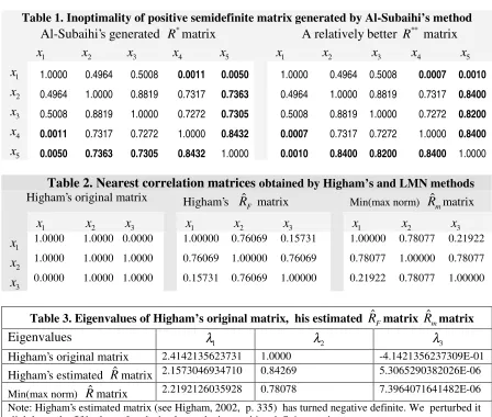
Table 1. Inoptimality of positive semidefinite matrix generated by Al-Subaihi’s method

Al-Subaihi’s generated R*matrix A relatively better R** matrix

1

x x₂ x₃ x₄ x₅ x₁ x₂ x₃ x₄ x₅

1

x 1.0000 0.4964 0.5008 0.0011 0.0050 1.0000 0.4964 0.5008 0.0007 0.0010

2

x 0.4964 1.0000 0.8819 0.7317 0.7363 0.4964 1.0000 0.8819 0.7317 0.8400

3

x 0.5008 0.8819 1.0000 0.7272 0.7305 0.5008 0.8819 1.0000 0.7272 0.8200

4

x 0.0011 0.7317 0.7272 1.0000 0.8432 0.0007 0.7317 0.7272 1.0000 0.8400

5

x 0.0050 0.7363 0.7305 0.8432 1.0000 0.0010 0.8400 0.8200 0.8400 1.0000

Table 2. Nearest correlation matrices obtained by Higham’s and LMN methods Higham’s original matrix _Higham’s ˆ

F

R matrix Min(max norm) Rˆ_mmatrix

1

x x₂ x₃ x₁ x₂ x₃ x₁ x₂ x₃

1

x 1.0000 1.0000 0.0000 1.00000 0.76069 0.15731 1.00000 0.78077 0.21922

2

x 1.0000 1.0000 1.0000 0.76069 1.00000 0.76069 0.78077 1.00000 0.78077

3

x 0.0000 1.0000 1.0000 0.15731 0.76069 1.00000 0.21922 0.78077 1.00000

Table 3. Eigenvalues of Higham’s original matrix, his estimated Rˆ_Fmatrix Rˆ_mmatrix

Eigenvalues λ₁ λ₂ λ₃

Higham’s original matrix 2.4142135623731 1.0000 -4.1421356237309E-01

Higham’s estimated Rˆmatrix 2.1573046934710 0.84269 5.3065290382026E-06

Min(max norm) Rˆmatrix 2.2192126035928 0.78078 7.3964071641482E-06

Note: Higham’s estimated matrix (see Higham, 2002, p. 335) has turned negative definite. We perturbed it slightly on the fifth place after decimal to make it a positive definite matrix.

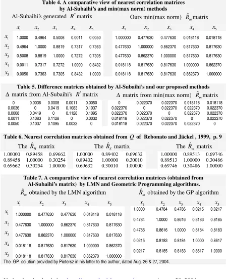
Table 4. A comparative view of nearest correlation matrices by Al-Subaihi’s and min(max norm) methods

Al-Subaihi’s generated R*matrix _{Ours min(max norm) ˆ}

m

R matrix

1

x x₂ x₃ x₄ x₅ x₁ x₂ x₃ x₄ x₅

1

x _{1.0000 0.4964 0.5008 0.0011 0.0050 1.000000 0.477630 0.477630 0.018118 0.018118}

2

x _{0.4964 1.0000 0.8819 0.7317 0.7363 0.477630 1.000000 0.862370 0.817630 0.817630}

3

x _{0.5008 0.8819 1.0000 0.7272 0.7305 0.477630 0.862370 1.000000 0.817630 0.817630}

4

x _{0.0011 0.7317 0.7272 1.0000 0.8432 0.018118 0.817630 0.817630 1.000000 0.862370}

5

x _{0.0050 0.7363 0.7305 0.8432 1.0000 0.018118 0.817630 0.817630 0.862370 1.000000}

Table 5. Difference matrices obtained by Al-Subaihi’s and our proposed methods

∆ matrix from Al-Subaihi’s R*matrix ∆ matrix from min(max norm) ˆR_mmatrix

0 0.0036 0.0008 0.0011 0.0050 0 0.022370 0.022370 0.018118 0.018118 0.0036 0 0.0419 0.1083 0.1037 0.022370 0 0.022370 0.022370 0.022370 0.0008 0.0419 0 0.1128 0.1095 0.022370 0.022370 0 0.022370 0.022370 0.0011 0.1083 0.1128 0 0.0032 0.018118 0.022370 0.022370 0 0.022370 0.0050 0.1037 0.1095 0.0032 0 0.018118 0.022370 0.022370 0.022370 0

Table 6. Nearest correlation matrices obtained from Q of Rebonato and Jäckel , 1999, p. 9

The ˆR_H matrix The ˆR_S martix The ˆR_m matrix

1.00000 0.89458 0.69662 1.00000 0.89402 0.69632 1.00000 0.89513 0.69746 0.89458 1.00000 0.30254 0.89402 1.00000 0.30010 0.89513 1.00000 0.30486 0.69662 0.30254 1.00000 0.69632 0.30010 1.00000 0.69746 0.30486 1.00000

Table 7. A comparative view of nearest correlation matrices (obtained from Al-Subaihi’s matrix) by LMN and Geometric Programming algorithms. ˆ

m

R obtained by the LMN algorithm Rˆ_m obtained by the GP algorithm

1

x x₂ x₃ x₄ x₅ x₁ x₂ x₃ x₄ x₅

1

x

1.000000 0.477630 0.477630 0.018118 0.018118

1.0000 0.4784

0.4786

0.0215

0.0217

2

x

0.477630 1.000000 0.862370 0.817630 0.817630

0.4784 1.0000 0.8616

0.8183

0.8185

3

x _{0.477630 0.862370 1.000000 0.817630 0.817630} 0.4786 0.8616 1.0000 0.8184 0.8183

4

x _{0.018118 0.817630 0.817630 1.000000 0.862370} 0.0215 0.8183 0.8184 1.0000 0.8617

5

x

0.018118 0.817630 0.817630 0.862370 1.000000

0.0217 0.8185 0.8183 0.8617 1.0000

The GP solution provided by Pietersz in his letter to the author, dated Aug. 26 & 27, 2004.

C -PROGRAM LMN

---C RANDOM WALK METHOD TO FIND Min(max norm) Nearest Positive C definite Marix from a given Negative Semidefinite Matrix

C --- INTEGER *2 IU,IV

DOUBLE PRECISION A(10),R(10),AR(10),XO(10,10),AA(10) DOUBLE PRECISION V(10,10),W(10,10),P(10),D,RH(10,10)

DOUBLE PRECISION SUML,LAMBDA,EPS,F,VO,VR,VOO,RAND,CN, RNORM DIMENSION MM(10)

CHARACTER *11 OFIL,IFIL

C PARAMETERS --- MAY BE CHANGED --- C EPS=ITERATIVE ACCURACY: EPSL=MAIN DIAGONAL ACCURACY C NITR=NO. OF TRIALS FOR RANDOM WALK SEARCH

C ITMAX=MAX NO. OF ITERATION FOR CONVERGENCE EPS= 0.00001

EPSL=0.00001 NITR=3

ITMAX=100

C Increase in NITR slows down program but gives better results WRITE(*,*)'FEED M and INPUT FILE NAME'

WRITE(*,*)'(M is the order of the input square matrix' WRITE(*,*)'INPUT FILE NAME in single quotes)'

READ(*,*) M,IFIL OPEN(7,FILE=IFIL) DO 1 I=1,M

1 READ(7,*)(XO(I,J),J=1,M) CLOSE(7)

WRITE(*,*)'FEED SEED TO GENERATE RANDOM NUMBERS'

WRITE(*,*)'(SEED lies between -32767 AND 32767, avoid zero)' READ(*,*) IU

WRITE(*,*)'OUTPUT FILE ? ' READ(*,*) OFIL

VOO=10.0**10 LTRY=0

ICO=1

CALL CONS(XO,P,M,ICO)

WRITE(*,*)'EIGEN VALUES OF THE ORIGINAL MATRIX XO ARE :' WRITE(*,*)(P(I),I=1,M)

PAUSE 'STRIKE ENTER TO PROCEED' DO 70 I=1,M

IF(P(I).LT.0.0) GOTO 90 70 CONTINUE

WRITE(*,*)'ALL EIGEN VALUES ARE NON-NEGATIVE' STOP

C ======================================================== 90 WRITE(*,*)'SOME EIGEN VALUES ARE NEGATIVE'

WRITE(*,*)'THE R MATRIX AT THIS STAGE IS : ' OPEN(8,FILE=OFIL, STATUS='NEW')

DO 789 I=1,M C P(I)=1.0

789 WRITE(8,89)(RH(I,J),J=1,M) CLOSE(8)

DO 788 I=1,M

788 WRITE(*,89)(RH(I,J),J=1,M) ITEST=0

DO 71 I=1,M

IF(P(I).LE.0.0) P(I)=RAND(IU,IV) F=F+P(I)

71 CONTINUE DO 72 I=1,M

72 P(I)=DABS(P(I)/F*M)

WRITE(*,*)'EIGEN VALUES ARE FORCED TO BE ALL POSITIVE' SUML=0.0

DO 78 I=1,M 78 SUML=SUML+P(I)

WRITE(*,*)(P(I),I=1,M),' SUM = ',SUML DO 999 IIT=1,NITR

LAMBDA=20.0

C Initialisation of decision variables DO 7 I=1,M

7 A(I)=DABS(P(I)) ICO=2

CALL CONS(RH,P,M,ICO)

C --- FUNCTION EVALUATION --- F=0.0

DO 11 I=1,M DO 11 J=1,M

D=DABS(XO(I,J)-RH(I,J)) IF(D.GT.F) F=D

11 CONTINUE VO=F

C --- IT=0

200 IT=IT+1

IF(IT.GT.1000) THEN

WRITE(*,*)'NO CONVERGENCE IN 1000 ITERATIONS' GOTO 1000

ENDIF

LAMBDA=LAMBDA/2.0 IMP=0

DO 100 II=1,ITMAX

C GENERATE M UNIFORMLY DISTRIBUTED RANDOM NUMBERS (-1,1) 150 DO 2 I=1,M

2 R(I)=2.0*(RAND(IU,IV)-0.5)

C NORMALISE THE RANDOM NUMBERS RNORM=0.0

DO 3 I=1,M

3 RNORM=RNORM+R(I)**2 RNORM=DSQRT(RNORM)

IF(RNORM.GT.1.0) GOTO 150 DO 4 I=1,M

4 R(I)=R(I)/RNORM

C ADD RANDOM NUMBERS TIMES LAMBDA TO A VECTOR DO 5 I=1,M

AR(I)=A(I)+LAMBDA*R(I) AR(I)=DABS(AR(I)) 5 CONTINUE

C --- FUNCTION EVALUATION --- CN=0.0

SUML=0.0 DO 74 I=1,M AR(I)=AR(I)/CN*M SUML=SUML+AR(I) 74 CONTINUE

C WRITE(*,*) 'SUML = ',SUML ICO=2

CALL CONS(RH,AR,M,ICO) F=0.0

DO 13 I=1,M DO 13 J=1,M

D=DABS(XO(I,J)-RH(I,J)) IF(D.GT.F) F=D

13 CONTINUE VR=F

C --- IF(VR.LT.VO) THEN

VO=VR DO 6 I=1,M A(I)=AR(I) 6 CONTINUE IMP=1 ENDIF 100 CONTINUE

IF((IMP.EQ.0).OR.(LAMBDA.GT.EPS)) GOTO 200 1000 CONTINUE

IF(VOO.GT.VO) THEN VOO=VO

DO 998 I=1,M AA(I)=A(I) 998 CONTINUE ENDIF 999 CONTINUE DO 997 I=1,M A(I)=AA(I) 997 CONTINUE VO=VOO SUML=0.0 DO 77 I=1,M SUML=SUML+A(I) 77 CONTINUE

WRITE(*,*)'SMALLEST MAX DEVIATE = ',VO WRITE(*,*)' '

WRITE(*,*)' TRIAL NUMBER = ',LTRY WRITE(*,*)' '

DO 152 I=1,M

IF(DABS(RH(I,I)-1.00).GT.EPSL) THEN RH(I,I)=1.0

ITEST=1 ENDIF 152 CONTINUE

IF(ITEST.EQ.1) THEN CALL CONS(RH,AR,M,1) LTRY=LTRY+1

VOO=10.0**10 GOTO 90

Write(*,*)' --- Convergence achieved ---' write(*,*)' '

WRITE(*,*)' NAME THE OUTPUT FILE TO STORE THE RESULT' WRITE(*,*)' (OUTPUT FILE NAME IN SINGLE QUOTES)' WRITE(*,*)'ESTIMATED MATRIX'

OPEN(8,FILE=OFIL, STATUS='NEW') DO 75 I=1,M

C RH(I,I)=1.00

WRITE(*,89)(RH(I,J),J=1,M) WRITE(8,89)(RH(I,J),J=1,M) 75 CONTINUE

CLOSE(8)

89 FORMAT(1X,6D13.5)

WRITE(*,*)'RESULTING MATRIX STORED IN FILE = ',OFIL

WRITE(*,*)'RUN THIS PROGRAM ONCE MORE ON ITS OWN OUTPUT FILE' WRITE(*,*)'UNTIL IT SAYS ALL EIGENVALUES ARE NON-NEGATIVE' END

C --- SUBROUTINE CONS(A,P,M,ICO)

C Constructs Matrix from its eigenvectors and values

DOUBLE PRECISION A(10,10),B(10,10),V(10,10),W(10,10),P(10),F DIMENSION MM(10)

IF(ICO.GT.1) GOTO 100 NN=1

1000 NADJUST=0 DO 10 I=1,M DO 10 J=1,M B(I,J)=A(I,J) 10 CONTINUE

CALL EIGEN(A,M,NN,V,W,P,MM)

C ==================================================== C NORMALIZATION OF EIGEN VECTORS

DO 50 I=1,M P(I)=0.0 P(I)=A(I,I) F=0.0

DO 51 J=1,M

51 F=F+V(J,I)*V(J,I) F=DSQRT(F)

DO 52 J=1,M V(J,I)=V(J,I)/F 52 CONTINUE

50 CONTINUE DO 11 I=1,M DO 11 J=1,M A(I,J)=B(I,J) 11 CONTINUE RETURN

C ===================================================== 100 DO 34 J=1,M

DO 341 JJ=1,M 341 W(J,JJ)=0.0 W(J,J)=P(J) 34 CONTINUE

C WRITE(*,*)'NOW W IS THE DIAGONAL L MATRIX' DO 36 J=1,M

DO 37 I=1,M

37 F=F+V(I,J)*V(I,J) DO 36 I=1,M

IF(P(J).EQ.0.0) THEN V(I,J)=0.0

ELSE

V(I,J)=V(I,J)/DSQRT(F/P(J)) ENDIF

36 CONTINUE DO 35 J=1,M DO 35 JJ=1,M A(J,JJ)=0.0 DO 35 I=1,M

A(J,JJ)=A(J,JJ)+V(J,I)*V(JJ,I) 35 CONTINUE

C WRITE(*,*)'NOW A IS V*L*VT MATRIX' RETURN

END

C --- SUBROUTINE EIGEN(A,N,NN,V,W,P,MM)

C Computes eigenvalues and vectors of a real symmetrix matrix DOUBLE PRECISION A(10,10),V(10,10),W(10,10),P(10)

DOUBLE PRECISION PMAX,EPLN,TAN,SIN,COS,AI,TT,TA,TB DIMENSION MM(10)

C --- INITIALISATION --- DO 50 I=1,N

DO 51 J=1,N V(I,J)=0.0 51 W(I,J)=0.0 P(I)=0.0 50 CONTINUE PMAX=0 EPLN=0 TAN=0 SIN=0 COS=0 AI=0 TT=0

EPLN=1.0D-310

C --- IF(NN.NE.0) THEN

DO 3 I=1,N DO 3 J=1,N V(I,J)=0.0

IF(I.EQ.J) V(I,J)=1.0 3 CONTINUE

ENDIF 2 NR=0 5 MI=N-1 DO 6 I=1,MI P(I)=0.0 MJ=I+1 DO 6 J=MJ,N

IF(P(I).GT.DABS(A(I,J))) GO TO 6 P(I)=DABS(A(I,J))

7 DO 8 I=1,MI

IF(I.LE.1) GOTO 10 IF(PMAX.GT.P(I)) GOTO 8 10 PMAX=P(I)

IP=I JP=MM(I) 8 CONTINUE

C EPLN=DABS(PMAX)*1.0D-09 IF (PMAX.LE.EPLN) THEN

C WRITE(*,*)'PMAX EPLN',PMAX, EPLN C PAUSE'CONVERGENCE CRITERION IS MET' GO TO 12

ENDIF NR=NR+1

C WRITE(*,*)'PMAX, EPLN',PMAX,EPLN 13 TA=2.0*A(IP,JP)

TB=(DABS(A(IP,IP)-A(JP,JP))+

1DSQRT((A(IP,IP)-A(JP,JP))**2+4.0*A(IP,JP)**2)) C WRITE(*,*) 'TA TB = ',TA,TB

TAN=TA/TB

C WRITE(*,*) 'TAN = ',TAN

IF(A(IP,IP).LT.A(JP,JP)) TAN=-TAN 14 COS=1.0/DSQRT(1.0+TAN**2)

SIN=TAN*COS AI=A(IP,IP)

A(IP,IP)=(COS**2)*(AI+TAN*(2.0*A(IP,JP)+TAN*A(JP,JP))) A(JP,JP)=(COS**2)*(A(JP,JP)-TAN*(2.0*A(IP,JP)-TAN*AI)) A(IP,JP)=0.0

IF(A(IP,IP).GE.A(JP,JP)) GO TO 15 TT=A(IP,IP)

A(IP,IP)=A(JP,JP) A(JP,JP)=TT

IF(SIN.GE.0) GO TO 16 TT=COS

GO TO 17 16 TT=-COS

17 COS=DABS(SIN) SIN=TT

15 DO 18 I=1,MI

IF(I-IP) 19, 18, 20 20 IF(I.EQ.JP)GO TO 18 19 IF(MM(I).EQ.IP) GO TO 21 IF(MM(I).NE.JP) GO TO 18 21 K=MM(I)

TT=A(I,K) A(I,K)=0.0 MJ=I+1 P(I)=0.0 DO 22 J=MJ,N

IF(P(I).GT.DABS(A(I,J))) GO TO 22 P(I)=DABS(A(I,J))

DO 23 I=1,N

IF(I-IP) 24, 23, 25 24 TT=A(I,IP)

A(I,IP)=COS*TT+SIN*A(I,JP)

IF(P(I).GE.DABS(A(I,IP))) GO TO 26 P(I)=DABS(A(I,IP))

MM(I)=IP

26 A(I,JP)=-SIN*TT+COS*A(I,JP)

IF(P(I).GE.DABS(A(I,JP))) GO TO 23 30 P(I)=DABS(A(I,JP))

MM(I)=JP GO TO 23

25 IF(I.LT.JP) GO TO 27 IF(I.GT.JP) GO TO 28 IF(I.EQ.JP) GO TO 23 27 TT=A(IP,I)

A(IP,I)=COS*TT+SIN*A(I,JP)

IF(P(IP).GE.DABS(A(IP,I))) GO TO 29 P(IP)=DABS(A(IP,I))

MM(IP)=I

29 A(I,JP)=-TT*SIN+COS*A(I,JP)

IF(P(I).GE.DABS(A(I,JP))) GO TO 23 GO TO 30

28 TT=A(IP,I)

A(IP,I)=TT*COS+SIN*A(JP,I)

IF(P(IP).GE.DABS(A(IP,I))) GO TO 31 P(IP)=DABS(A(IP,I))

MM(IP)=I

31 A(JP,I)=-TT*SIN+COS*A(JP,I)

IF(P(JP).GE.DABS(A(JP,I))) GO TO 23 P(JP)=DABS(A(JP,I))

MM(JP)=I 23 CONTINUE

IF(NN.EQ.0) GOTO 7 DO 32 I=1,N

TT=V(I,IP)

V(I,IP)=TT*COS+SIN*V(I,JP) V(I,JP)=-TT*SIN+COS*V(I,JP) 32 CONTINUE

GO TO 7 12 RETURN END

C --- FUNCTION RAND(IU,IV)

C Generates Rectangular (0,1) Random Numbers DOUBLE PRECISION RAND

INTEGER *2 IU,IV IV=IU*259

IF(IV.GE.0) GOTO 2 IV=IV+32767+1 2 RAND=IV

IU=IV

RAND=RAND*0.3051851E-04 RETURN