Munich Personal RePEc Archive
Neuro-dynamic programming for the
efficient management of reservoir
networks
de Rigo, Daniele and Rizzoli, Andrea Emilio and
Soncini-Sessa, Rodolfo and Weber, Enrico and Zenesi, Pietro
Dipartimento di Elettronica e Informazione, Politecnico di Milano,
Italy, IDSIA, Manno, Switzerland
December 2001
Online at
https://mpra.ub.uni-muenchen.de/42233/
Copyright © 2001 The Modelling and Simulation Society of Australia and New Zealand Inc. (MSSANZ). This is the author's version of the work.
See:
http://www.mssanz.org.au/documents/MODSIMPapersToJournalPapers-MSSANZGuidelines.pdf
The definitive version was published in the proceedings of MODSIM 2001 International Congress on Modelling and Simulation. “Integrating Models for Natural Resources Managment Across Disciplines, Issues and Scales”. Modelling and Simulation Society of Australia and New Zealand, December 2001
http://www.mssanz.org.au/MODSIM01/MODSIM01.htm
Cite as:
de Rigo, D., Rizzoli, A.E., Soncini-Sessa, R., Weber, E., Zenesi, P. (2001). Neuro-dynamic programming for the efficient management of reservoir networks. Proceedings of MODSIM 2001 International Congress on Modelling and Simulation. Modelling and Simulation Society of Australia and New Zealand. December 2001, Vol. 4, pp. 1949–1954. ISBN: 0-867405252.
Neuro-Dynamic Programming for the Efficient
Management of Reservoir Networks
D. de Rigoa
, A. E. Rizzolib
, R. Soncini-Sessaa
, E. Webera
, P. Zenesia
a
Dipartimento di Elettronica e Informazione, Politecnico di Milano, Italy
b IDSIA, Manno, Switzerland ([email protected])
Abstract: The management of a water reservoir can be improved thanks to the use of stochastic dynamic programming (SDP) to generate management policies which are efficient with respect to the management objectives (flood protection, water supply for irrigation and hydropower generation, respect of minimum envi-ronmental flows, etc.). The improvement in efficiency is even more remarkable when the problem involves a reservoir network, that is a set of reservoirs which are interconnected. Unfortunately, SDP is affected by the “curse of dimensionality” and computing time and computer memory occupation can quickly become unbear-able. Neuro-dynamic programming (NDP) can sensibly reduce the demands on computer time and memory thanks to the approximation of Bellman functions with Artificial Neural Networks (ANNs). In this paper an application of neuro-dynamic programming to the problem of the management of reservoir networks is pre-sented.
Keywords: Water reservoir management; Stochastic dynamic programming; Neuro-dynamic programming.
1. INTRODUCTION
The management of water quantity has considera-bly profited from the advent of computers and the application of Operations Research and Systems Analysis methodologies to solve the problem of finding the optimal release of water in order to satisfy demand for hydropower generation, agri-cultural and urban use, and to satisfy environ-mental constraints. One of the most successful techniques has been Dynamic Programming [Bell-man and Dreyfus, 1959] and various authors have applied the methodology to water management. Unfortunately, from the very beginning it was ap-parent that an increase of the dimensionality of the problem, i.e. an addition of reservoirs, caused an exponential increase in the time required to find a solution. This problem was named the “curse of dimensionality” by Bellman and prevented the ap-plication of the methodology to real world water systems consisting of more than two or three reser-voirs. Recently, Bertsekas and Tsitsiklis (1996) have proposed a methodology, named neuro-dynamic programming, based on the functional approximation of the Bellman function using Arti-ficial Neural Networks (ANNs). The ANN-based approximation can be obtained exploring
thedis-cretisation grid of the search space with a lower resolution, thus reducing the time required to solve one step of the Bellman equation.
In this paper we present an application of this methodology to the solution of the problem of op-timal water management. We have implemented an extension to the Successive Approximation Al-gorithm which has been already adapted to the case of reservoir management policy design [Piccardi and Soncini, 1991].
We finally report some preliminary experimental tests
2. THE PROBLEM
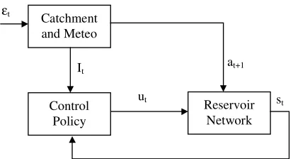
Since the first pioneering works by Maas (1962), the problem of the management of a regulated lake has been represented with a feedback control scheme with feedforward compensation (Figure 1).
and the catchment state. Both these systems are affected by a stochastic disturbance εt.
[image:4.595.86.293.114.226.2]Control Policy Reservoir Network Catchment and Meteo εt It ut at+1 st
Figure 1. Closed loop control scheme with feed-forward compensation.
According to the chosen modelling representation, the components of the vector It can be, e.g., the piezometric head of groundwater, the reservoir inflow during the 24 hours preceding the release decision (at+1); the stochastic disturbance εt can be, e.g., the atmospheric pressure, the solar radiation, the rainfall.
The control policy can be determined as the solu-tion of an optimal control problem defined as fol-lows. The reservoir is represented by the mass conservation equation: ) , , ( 1 1 1
1 + + +
+ = t + t − t t t t
t s a r s u a
s (1)
where rt+1 is the actual release in the interval [t, t+1).
The meteorological system and the catchment are the most difficult component to model, because of the complexity of the meteorological and hydro-logical processes. Very often only the catchment is considered and the reservoir inflow at+1 is repre-sented by simple stochastic autoregressive models of order q.
) , ,..., ,
( t 1 t 2 t q t
t
t a a a
a =χ − − − ε (2)
where εt is a white gaussian noise. Here
| ,..., ,
| t 1 t 2 t q
t a a a
I = − − − .
The model of the whole dynamic system, com-posed of the meteorological system, the catchment and the reservoir, can thus be represented in the compact vectorial equation:
) , ,
( 1
1 +
+ = t t t t
t f x u
x ε (3)
where xt is the state vector, composed by the state variables in st, and It. Because of climate periodic-ity, the function ft(⋅,⋅,⋅)is periodic of period T equal to one year.
During the system evolution, the state transition from xt to xt+1 can produce an instantaneous cost, expressing the lack of fulfillment of management objectives, computed as the weighted sum of the costs associated with the k objectives:
t t k
j j
t w g
g = ∑
=1
(4)
where wjis the weight of the j-th objective. Also the step costs are periodic of period T.
We define as policy the infinite sequence
} , , {m0 m1K
p= of periodic functions of period T
where:
) ( t
t
t m x
u = (5)
The optimal control problem is to find the policy that minimises a functional of the costs in the fu-ture, over an infinite horizon. Using the Laplace criterion (use of the expected value operator on the disturbance ε), given an initial state x0 and a dis-count rate α for the future costs, the cost functional of a given policy p is defined as:
)] , , ( [ lim ) , ( 1 0 ... 0 1 1 + = ∞ → ∑ = + t t t t t h t h u x g E p x J h ε α ε ε
The optimal control problem is therefore solved when we find the policy po
which minimises: ) , ( min )
(x0 J x0 p J p = (6a) subject to: ) , , ( 1 1 +
+ = t t t t
t f x u
x ε (6b)
) , | ( t 1 t t
t
t ∼Φ ε + x u
ε (6c)
t
t S
x ∈ ut ∈Ut(xt) εt ∈Dt (6d)
) ( t
t
t m x
u = (6e)
where St,Ut,Dtare the discretised domains of the
state, control and disturbance.
3. THE SOLUTION BASED ON STOCHASTIC DYNAMIC PROGRAMMING
The solution of the optimal control problem (6a-6e) by SDP is based on the evaluation of the opti-mal cost-to-go, which is defined as the cost that one would have to pay if the system would be ini-tially in state xt+1 and the system’s future trajectory would be obtained applying optimal control deci-sions in every state transition. We name this cost
) ( 1 1 + + t o t x
H . If the optimal cost-to-go would be
) ( t
o
t x
m at time t would be easily found minimising the expected value of the present cost and the dis-counted optimal cost-to-go:
(
)
( )
] , , [ E min arg ) ( 1 1 1 1 + + + + = + t o t t t t t u t o t x H u x g x m t t α ε ε (7)The optimal cost-to-go associated with the present state is therefore given by the following recursive equation:
(
, ,)
( )
] [ E min )( 1 1 1
1 + + + + = + t o t t t t t u t o
t x g x u H x H t t α ε ε (8)
which is known as the Bellman equation and its solution is the Bellman function.
Under the previous hypotheses, it can be shown that the Bellman function is a periodic function, of period T, which can be obtained using the Succes-sive Approximations Algorithm (SAA) [Bertsekas, 1995] that, proceeding backwards in time from T to 1, solves the recursive equation (8) verifying the constraints (6b-6e).
To determine the right hand side of equation (8), the algorithm, for each value of xt, must explore all the possible values of ut and of εt. Since this algo-rithm operates on a discrete search space, we have always implicitly assumed that the domains of u, x and ε were discrete. Actually, it is up to the system analyst to find a satisfactory discretisation of the continuous domains of these variables. The choice of the discretisation is fundamental since it reflects on the algorithm complexity which is combinato-rial in the number of states, controls and in their discretisations. If we assume to have n states, each one discretised into N classes, the computational cost of SDP is proportional to:
T
Nn× (9)
where T is the number of time steps.
In other words, if we increase the resolution of the discretisation, thus enhancing the adherence of our model to the real world, or if we consider more controls and states, to describe more complex res-ervoir networks, it may happen that the time re-quired to compute a policy becomes excessively long.
Many methods have been devised to overcome this limitation. Georgakakos and Marks (1987, 1989) proposed the Extended Linear Quadratic Gaussian method, an approach based on the Pontriagyn’s Maximum principle which does not resent of the dimensionality problem, but requires the cost func-tional to be a quadratic function. Another approach is the one proposed by Nardini and Soncini-Sessa (1994). They developed an heuristic control scheme, named Partial Open Loop Feedback
Con-trol, based on the substitution of the off-line control problem with a succession of simpler problems, which is effective in presence of a detailed de-scription of the stochastic part of the water system.
In the following, we introduce a new approach based on neuro-dynamic programming [Bertsekas and Tsitsiklis, 1996] which has the advantage of retaining the ability of SDP to deal with highly non-linear problems, while reducing the algorithm complexity thanks to the approximation of the Bellman functions via ANNs.
3. THE SOLUTION BASED ON NEURO-DYNAMIC PROGRAMMING
As previously seen, the main problem with SDP lies in the dimensions of the search space, if it is too big, it is nearly impossible to find a solution in a reasonable time. Unfortunately water systems with three or more reservoirs are quite common and each reservoir is modelled with one state vari-able. It is therefore very easy to come to a point where the discretisation grid of the state variables must be so loose in order to have a computationally solvable problem that the resulting policy is practi-cally unusable.
Another critical factor is the requirement of mem-ory space: for a network with three reservoirs, each state discretised on a grid with 1000 points, under the simplifying assumption that the reservoir in-flows are described by gaussian noise (which does not add to the state dimensions), one would need 1.14 Terabytes of memory space to store the Bell-man function values in single precision only.
A solution to overcome these limitations is to use an approximation H~ of the Bellman Function
) (⋅
⋅o
H to represent the behaviour of the original
function interpolating from a limited subset Stof points extracted from discretisation grid St, so that
t t
t S S
x ∈ ⊂ . Since computing a point of H⋅o(⋅) is computationally very expensive, in terms of both CPU time and memory space, reducing the number of computed points will be extremely beneficial.
In the next sections, first we introduce Artificial Neural Networks as function approximators, then we explain how the Bellman function approxima-tions can be used in an algorithm that differs only slightly from the original SAA.
3.1. Approximating the Bellman Function
1989, Kreinovich 1991]. This means that an ANN can approximate any function to any desired de-gree of accuracy provided that a sufficient number of hidden units are used, and thus we can approxi-mate an highly nonlinear map H(x), such as the Bellman function, where x is a vector, with a feed-forward network H~(x,ϑ), where ϑis the vector of weights on the arcs connecting the network layers.
The objective is to find a network structure (num-ber of hidden layers, num(num-ber of neurons) so that the vector ϑcan be efficiently computed, while retaining a “good” approximation ability, thus ena-bling H~(x,ϑ) to be a compact representation of H(x).
Note that the dimension of vector ϑ is equal to r = s(n+2)+1 where s is the number of neurons and n the dimension of the state. Thus, to store T ap-proximations of a Bellman function, we only need to store rT values. In the case of the network with three reservoirs, using a feedforward ANN with 3 neurons in the hidden layer (which are enough to approximate the Bellman functions in our experi-mental cases), leads to the requirement of only 216 Kilobytes of memory space, as opposed to the 1.14 Tb with traditional SDP.
The improvement is not so remarkable when we deal with CPU time, since ANNs must be trained.
Input
Layer Hidden Layer
Output Layer
x1
x2
x3
y1
y2
[image:6.595.88.281.417.553.2]y3
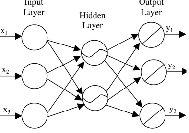
Figure 2. A typical feedforward network.
3.2. Training the Bellman function approxi-mations
In a feedforward ANN neurons are organised in layers: the input layer is directly connected with the inputs, the output layer takes the outputs of the hidden layer (one, or more) and produces the net-work output.
In Figure 2 we have represented a network with three inputs and three outputs, but the Bellman function approximators will always have n inputs, where n is the number of state variables, and a sin-gle output (the cost-to-go value).
The input layer (the empty token in Figure 2) sim-ply distributes the input values to the hidden layer weighting the importance of the connections. The weighted inputs are then processed by each node in the hidden layer thanks to an activation function. The output of the hidden layer is either passed on to a next hidden layer or sent to the output nodes where it is weighted and processed by a (usually) linear activation function. When all the activation functions are linear, also in the hidden layers, the ANN can be reduced to a linear filter and can be trained using a standard least squares algorithm. ANN show their ability to approximate highly non-linear functions when the activation functions are non-linear. We have chosen to use an hyperbolic tangent as activation function. Unfortunately the least squares algorithm does not work anymore and therefore the backpropagation algorithm has been invented by [Rumelhart et al. 1986]. It minimises the output error of the network (10), given by the sum of squared errors between the target to and the network output yo:
∑ −
=
o o o P t y
E ( )2
2 1
(10)
The error is minimised computing its derivative with respect to the weights and then applying the forward and backward passes of the backpropaga-tion algorithm to express the weight gradient as a function of the network inputs for each layer.
In the backpropagation algorithm the main prob-lem is the descent of the weight gradient and re-search has focused on the development of gradient descent algorithms which would converge quickly and avoiding local minima. Most of the time re-quired training a network is spent in these compu-tation, where the trade-off is between accuracy and computational complexity, since most accurate algorithms require the inversion of the Jacobian and the Hessian of the weight matrices of consider-able dimensions. Currently we have implemented the Levenberg-Marquardt algorithm [Hagan and Menhaj, 1996] which has been designed to ap-proach the speed of second-order methods without having to compute the Hessian.
3.3. The NDP algorithm
Once an approximation architecture H~(x,ϑ)of H(x) has been found, the sub-optimal policy
) ( ~
t t x
m is given by [Bertsekas and Tsitsiklis,
1996]:
(
)
(
t t)
t t tt t t t u t
t
S S x x
u x g x
m
t t
⊂ ∈ ∀ +
=
+ + +
+
+
] , H~
, , [ E min arg ) ( ~
1 1 1 t
1
1
ϑ α
ε
Comparing equation (11) with (7), it appears that
( )
11 t
H~ + xt+ must be trained using Hto+1
( )
xt+1 as target and the vector xt+1 as pattern. We remark that the original Bellman function is not available, but we can exploit the recursive nature of the Bellman equation to generate the Bellman func-tions needed to train their approximafunc-tions thanks to the approximate DP formula:(
)
(
,)
]H~
, , [ E min ) ( ˆ
1 1 1 t
1
1
+ + +
+ +
=
+
t t
t t t t u t t
x u x g x
H
t t
ϑ α
ε
ε (12)
The left-hand side of (11) is an approximate cost-to-go function, which can be used to train
) , ( ~
t t t x
H ϑ , which, in turn, will be used in (11) to
obtain Hˆt−1(xt−1). It can be proven formally that if the approximation architecture is “good enough”, then Ht
~
is a close approximation of the optimal
cost-to-go functionHto. Bertsekas and Tsitsiklis
also show that in some particular cases, for some values of the discount rate α, there is still possibil-ity for algorithm divergence. Such a situation can be avoided limiting the class of approximators, but also limiting their power and ease of use.
The algorithm is therefore a simple rewriting of the orginal SAA:
Step 0) Initialisation. The current algorithm itera-tion index j is set to 0. Initialise H0<0>(⋅)=0 for
each state value. Train an ANN H~T(xT,ϑT) us-ing the discretisation grid of xt+1 as pattern and the identically null function H0<0>(⋅) as target.
Step 2) Main loop. For each algorithm iteration j compute backwards in time, for t from T-1 down to 0, T functions Hˆt<j>(⋅)using equation (11). At
each time step, after having obtained Hˆt<j>(⋅),
compute its approximation H~t<j>(⋅,ϑt) training the ANN. When t = 0, check if an appropriate convergency criterion, measuring the distance be-tween two Bellman functions at successive itera-tions, has been satisfied, if not, increment the it-eration index j and go back to the beginning of Step 2 after having set H0<j+1>(⋅)=HT<j>(⋅).
4. PRELIMINARY RESULTS
Currently, the algorithm we have presented in this paper has been applied only to some test cases to verify its correct functioning and get some first
results to understand how to extend its application to real world cases.
A first test was designed to verify the convergence of the algorithm and obtain some data on its theo-retical performance. The test case was a reservoir network with a single reservoir, fed by a catchment described as a white gaussian noise, and with an agricultural district with a give water demand, con-stant over the optimisation period. One step of the SDP algorithm, that is, the evaluation of the right hand side of equation (8) for all the possible values of xt, given the cardinality of Ut, card(Ut) = 7, card(Dt) = 10, card(St) = 17, took 0.97 seconds. One step of the NDP algorithm took 12.41 sec-onds, of which 0.29 seconds were spent to evaluate the right hand side of (8) for a given xt, while in the SDP case, the required time was only 0.058 sec-onds. Another 0.45 seconds were needed for each xt to train the ANN which approximated the Bell-man function obtained in the SDP case with an error less than 10-2. Note that NDP was applied using the same discretisation of the state space of the SDP case. The tests were performed on a Pentium II at 350 Mhz, running under Linux.
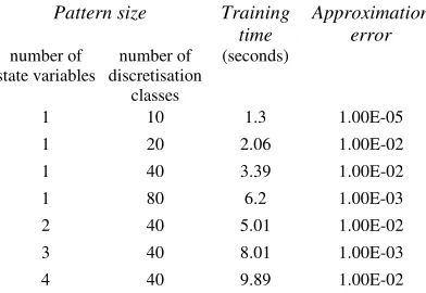
[image:7.595.322.518.518.653.2]We then performed some tests to understand how the training time for an ANN varies with the pat-tern dimension, which depends on the number of state variables (the dimension of the independent variable vector x in a function y = f(x)) and the number of points in the discretisation classes of each component of the vector. These results are reported in Table 1.
Table 1. Training times and approximation errors measured in the training of the functions y = ln(x)-sin(x) (1 state variable), y = ln(x) – sin(y) (2 vari-ables), y = ln(x) – sin(y+z) (3 variables), y = ln(x+y)-sin(z+w) (4 variables).
Pattern size Training time
Approximation error number of
state variables
number of discretisation
classes
(seconds)
1 10 1.3 1.00E-05
1 20 2.06 1.00E-02
1 40 3.39 1.00E-02
1 80 6.2 1.00E-03
2 40 5.01 1.00E-02
3 40 8.01 1.00E-03
4 40 9.89 1.00E-02
was closing down, thanks to the reduction of the state grid to 8 discretisation classes in the NDP case. We measured each an average time per itera-tion of 8 seconds in the SDP case, against 47.36 seconds for the NDP case. We are currently ex-perimenting NDP on a real world case, the synthe-sis of management policies for the Piave water system. No results are yet available as we write, since we are still setting up the experimental framework, but we expect to notice a considerable reduction in computing time, given that there are three state variables, with their discretisation classes equal to 102, 41 and 96 points. Sampling those classes, taking one point out of four, will allow to browse a search space of 6000 points in the NDP case against the 401472 points of the SDP case.
5. CONCLUSIONS
An approach to the management of reservoir net-works based on neuro-dynamic programming has been presented. Neuro-dynamic programming allows to reduce the amount of memory needed to store the Bellman functions during the solution of an optimal control problem. It also reduces the computation time when the state space, used as training pattern, is sampled with a coarser grid, while the ANN, which approximates the Bellman function, still manages to maintain a good ap-proximation performance.
The first results are promising, but there is space for more research, especially on the efficient sam-pling of the discretised state space, in order to ob-tain the most efficient approximation of the Bell-man function.
6. REFERENCES
Bellman, R.E., and Dreyfus, S.E., Functional ap-proximations and dynamic programming, Mathe-matical Tables and Other Aids to Computation, 13, pp. 247–251, 1959.
Bertsekas, D.P., and J.N. Tsitsiklis, Neuro-Dynamic Programming, Athena Scientific, Belmont, MA, 1996.
Georgakakos, A.P., and Marks, D.H., A new method for real-time operation of reservoir sys-tems, Water Resour. Res., 23(7), pp. 1376–1390. 1987.
Georgakakos, A.P., Extended Linear Quadratic Gaussian Control for the real-time operation of reservoir systems, in Dynamic Programming for Optimal Water Resources Systems Analysis, A. Esogbue, ed., Prentice Hall Publishing Company, NJ, pp. 329–360, 1989.
Hagan, M.T., and M. Menhaj, Training feedfor-ward networks with the Marquardt algorithm, IEEE Transactions on Neural Networks, 5(6), pp. 989–993, 1994.
Hornik, K., Multilayer feedforward networks are universal approximators, Neural Networks, 2, pp. 359–366, 1989.
Kreinovich, V., Arbitrary nonlinearity is sufficient to represent all functions by neural networks: a theorem, Neural Networks, vol.4, pp. 381–383, 1991.
Nardini, A, C. Piccardi and R. Soncini-Sessa, A decomposition approach to suboptimal control of discrete-time systems, Optimal Control Applica-tions and Methods, 15, pp. 1–12, 1994.
Piccardi, C. and R. Soncini-Sessa, Stochastic dy-namic programming for reservoir optimal control: dense discretization and inflow correlation as-sumption made possible by parallel computing. Water Resour. Res., 27(2), pp. 729–741, 1991.