Topological photonics with anisotropic materials

(1)

Topological Photonics with Anisotropic

Materials

Robert Mc Guinness

A thesis submitted for the degree of Doctor of Philosophy

in the

Quantum Light and Matter Group School of Physics

Trinity College Dublin

(2)

(3)

iii

Declaration

I declare that this thesis has not been submitted as an exercise for a degree at this or any other university and it is entirely my own work.

I agree to deposit this thesis in the University’s open access institutional reposi-tory or allow the library to do so on my behalf, subject to Irish Copyright Legislation and Trinity College Library conditions of use and acknowledgement.

I consent to the examiner retaining a copy of the thesis beyond the examining period, should they so wish (EU GDPR May 2018).

(4)

(5)

v

Summary

In this thesis we discuss and explore several different aspects of the topological classification of light propagating through matter, or topological photonics. In particular we will focus on anisotropic materials where the optical response is de-pendent on the polarisation and direction of propagation of the incoming light. We will consider both homogeneous dielectric media and periodically patterned optical materials known as photonic crystals. These explorations will consider either the weak-coupling regime, where the solutions of the wave equation describe photons, or the strong-coupling regime, where the solutions describe mixed light-matter quasiparticles called polaritons.

Our first subject is examining the topological characterisation of the refractive index surfaces of homogeneous optical materials. We do this by computing a topological invariant known as a Chern number in the case of different materials. The materials we consider are biaxial dielectrics with optical activity. In the absence of optical activity the refractive index surfaces of biaxial materials feature polari-sation degeneracies. The introduction of optical activity lifts these degeneracies. We explore whether in combination biaxiality and either of two possible forms of optical activity can produce optical topological order. We find that the refractive index surfaces of chiral biaxial materials can have non-zero Chern numbers. We additionally derive an effective Hamiltonian which paraxially evolves light through a biaxial optically active material in directions close to a lifted degeneracy.

Next we turn to periodically patterned optical materials. We adapt the derived Hamiltonian to describe anisotropic, optically active two dimensional photonic crystals of two differing patterning geometries. The two geometries which we consider are either a square or a triangular arrangement of the dielectric con-stituents. For each geometry we examine the topological phase diagrams for each of the two forms of optical activity as we vary relevant parameters. We find that, for each geometry and either form of optical activity, topologically non-trivial iso-frequency surfaces can be achieved. The results of the studies for each form of patterning is compared and contrasted with each other and with the homoge-neous material. We additionally explore the possibility of topological edge states for these anisotropic photonic crystals when they are considered in a finite geometry.

(6)

(7)

vii

Acknowledgements

Firstly I would like to thank my supervisor, Prof. Paul Eastham, for all his guidance and support. I have enjoyed the many lengthy and stimulating discussions we have had over the past four years. I am thoroughly indebted to him for what depth of understanding I have accrued during my postgraduate studies. Paul is a brilliant supervisor and it has been a privilege to work with him.

I am also thankful to the wider academic, technical and administrative com-munity within the school of physics. It has been a great place to carry out both undergraduate and postgraduate studies. In particular I would like to thank Prof. David O’Regan, Prof. John Donegan, Prof. David McCloskey and Prof. John Goold for helpful discussions over the course of my postgraduate studies.

The writing up process for this thesis has proved an acutely stressful experience. I was lucky to have resources and supports like the Student Learning Development and the Student Counselling Service to help me during this tough time.

(8)

the final months. Finally there is Laura M. who has been the best thing about my last nine months in Trinity. She has believed in me when I’ve found it hard to myself.

Although my tether to the campus is passing I will never be able to de-couple my feelings for Trinity from the friends with whom I shared the campus. As long as I hold on to them my personal Trinity will live on.

(9)

ix

List of Figures

1.1 Genus as a topological invariant . . . 4

1.2 Chern insulator vector field plot for three differentm . . . 8

1.3 Bulk band structure of Chern insulator for three differentm . . . 9

1.4 Finite geometry band structures for three differentm . . . 10

1.5 Edge state eigenvectors of Chern insulator . . . 10

1.6 Topological phase diagram of Weyl semi-metal lattice model . . . 15

1.7 Weyl points in the 3DBrillouin zone . . . 16

1.8 Fermi arc in Weyl semi-metal lattice model . . . 16

1.9 Real and imaginary parts of eigenvalues showing an exceptional point 18 1.10 Splitting of real and imaginary parts of eigenvalues as loss difference varied . . . 19

2.1 Refractive index surfaces of a homogeneous biaxial material . . . 35

2.2 Direction of linear polarisation on the biaxial index surfaces . . . 36

2.3 Alternative plot showing the direction of linear polarisation on the biaxial index surfaces . . . 37

2.4 Refractive index surfaces of a homogeneous biaxial material with op-tical activity . . . 38

2.5 Polarisation structure of a biaxial Faraday effect material on the re-fractive index surfaces . . . 39

2.6 Polarisation structure of a chiral biaxial material on the refractive in-dex surfaces I . . . 40

2.7 Polarisation structure of a chiral biaxial material on the refractive in-dex surfaces II . . . 41

2.8 Principal axes of the dielectric tensor and coordinate axes along optic axis . . . 44

3.1 Photonic crystals with varying dimensions of patterning. . . 51

3.2 Entrance face of a square 2D PhC . . . 52

3.3 Iso-frequency surfaces of a square PhC composed of biaxial material . 56 3.4 Schematic showing evolution of iso-frequency surfaces with period-icity and optical activity . . . 56

3.5 Vorticity plots of effective magnetic field at two differenta/λ. . . 58

(14)

3.7 Comparison between the C-point flow of lattice Hamiltonian to that of plane-wave simulation. . . 60 3.8 Comparison between iso-frequency surfaces generated from lattice

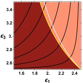
Hamiltonian with those generated from plane-wave simulation . . . . 62 3.9 Topological phase diagram of square PhC composed of biaxial

Fara-day effect material . . . 63 3.10 Effect of biaxiality on topological phases of square PhCs composed of

biaxial Faraday effect material . . . 66 3.11 Topological phase diagram of square PhCs composed of biaxial

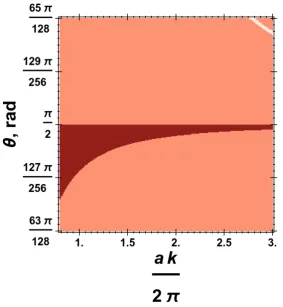
Fara-day effect material as cone semi-angle is continously varied . . . 67 3.12 Effect of lattice spacing to wavelength ratio on topological phases of

square PhCs composed of biaxial Faraday effect material . . . 68 3.13 Topological phase diagram of square PhCs composed of biaxial

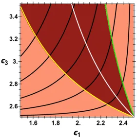
Fara-day effect material as lattice spacing to wavelength ratio is continu-osly varied . . . 69 3.14 Topological phase diagram of square PhCs composed of sphenoidal

or pedial chiral biaxial material . . . 74 3.15 Effect of biaxiality on topological phases of square PhCs composed of

chiral biaxial material . . . 75 3.16 Topological phase diagram of square PhCs composed of chiral biaxial

material as cone semi-angle is continously varied . . . 76 3.17 Effect of lattice spacing to wavelength ratio on topological phases of

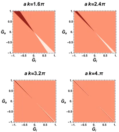
square PhCs composed of chiral biaxial material . . . 78 3.18 Topological phase diagram of square PhCs composed of chiral biaxial

material as the lattice spacing to wavelength ratio is continuously varied 79 3.19 Fraction of topologically non-trivial square PhCs with random chirality 80 4.1 Entrance face of a triangular 2D PhC . . . 84 4.2 First Brillouin zone of triangular lattice . . . 85 4.3 Iso-frequency surfaces of a triangular PhC composed of biaxial material 87 4.4 C-points of triangular PhCs from lattice Hamiltonian . . . 88 4.5 Parameter flow of C-points in triangular PhCs from lattice Hamiltonian 89 4.6 C-points of triangular PhC from lattice Hamiltonian at high paraxiality 90 4.7 Comparison between iso-frequency surfaces generated from lattice

Hamiltonian and those generated from plane-wave simulation for a triangular geometry . . . 91 4.8 Density plots of splittings of simulated iso-frequency surfaces over

the Brillouin zone at two different frequencies . . . 92 4.9 Topological phase diagram of triangular PhC composed of biaxial

Faraday effect material . . . 94 4.10 Effect of biaxiality on topological phases of triangular PhCs composed

(15)

xv

4.11 Topological phase diagram of triangular PhC composed of biaxial Faraday effect material as cone semi-angle is continuously varied . . . 97 4.12 Effect of lattice spacing to wavelength ratio on topological phase

dia-gram of triangular PhCs composed of biaxial Faraday effect material . 98 4.13 Topological phase diagram of triangular PhC composed of biaxial

Faraday effect material as lattice spacing to wavelength ratio is con-tinuously varied . . . 99 4.14 Topological phase diagram of triangular PhCs composed of

sphe-noidal or pedial chiral biaxial material . . . 102 4.15 Effect of biaxiality on topological phases of triangular PhCs composed

of chiral biaxial material . . . 104 4.16 Topological phase diagram of triangular PhCs composed of chiral

bi-axial material as cone semi-angle is continuously varied . . . 105 4.17 Effect of lattice spacing to wavelength ratio on topological phases of

triangular PhCs composed of chiral biaxial material . . . 106 4.18 Topological phase diagram of triangular PhC composed of chiral

bi-axial material as lattice spacing to wavelength ratio is continuously varied . . . 107 4.19 Comparison of topological phase diagrams between square and

trian-gular geometries . . . 108 4.20 Examination of geometrical anomalies in topological phase diagrams . 110 5.1 Two possible edge terminations of 2Dsquare lattice . . . 115 5.2 Absolute value of eigenvalue of discrete translation operator alongy

as band gap ink⊥is closed . . . 119 5.3 Bulk and finite geometry band structures as band gap ink⊥is closed . 120 5.4 Edge state densities as band gap ink⊥is closed . . . 121 5.5 Absolute value of eigenvalue of discrete translation operator alongy

as band gap inkk is closed . . . 122 5.6 Bulk and finite geometry band structures as band gap inkk is closed . 123 5.7 Edge state densities as band gap inkkis closed . . . 123 5.8 Three types of finite geometry considered . . . 125 5.9 Edge state densities in geometry that includes adjacent material . . . . 126 5.10 Absolute value of eigenvalue of discrete translation operator alongy

at finitek_k . . . 126 5.11 Absolute value of discrete translation operator alongyand edge state

densities in geometry that includes adjacent material. . . 127 5.12 Translation operator eigenvalue analysis of finite photonic crystal . . . 129 5.13 Finite geometry band structure of square patterned PhC composed of

chiral biaxial material . . . 130 5.14 Edge state density plots of finite square patterned PhC composed of

(16)

5.15 Finite geometry band structure in topologically trivial parameter regime131 6.1 Unit cell of zincblende lattice . . . 136 6.2 Schematic band structure of a zincblende semiconductor . . . 137 6.3 Simple polariton dispersion relation . . . 138 6.4 Dependence of exciton 1s energy levels on applied magnetic field

strength in the low-field regime . . . 146 6.5 Excitation structure of optically induced transitions . . . 149 6.6 Frequency dependence of GaAs dielectric tensor components close to

band edge . . . 151 6.7 Density plot of the discriminant in the absence of any resonance

broadening . . . 156 6.8 Bulk GaAs polariton dispersion for ˆkk ˆz . . . 157 6.9 Bulk GaAs polariton dispersion for ˆkk ˆzwith numbered degeneracies 158 6.10 First degeneracy in ˆkk ˆzpolariton dispersion . . . 159 6.11 Transverse dispersion through first degeneracy in ˆkk ˆzpolariton

dis-persion . . . 159 6.12 Degeneracies 2−5 in ˆkk ˆzpolariton dispersion . . . 160 6.13 Sixth degeneracy in ˆkk ˆzpolariton dispersion . . . 161 6.14 Transverse dispersion through sixth degeneracy in ˆk k ˆz polariton

(17)

xvii

List of Tables

2.1 Non-zero components of chirality tensor for non-centrosymmetric bi-axial crystals . . . 29 6.1 Material parameters of direct band gap semiconductors considered in

this work. The data is taken from Winkler [164] and Fu et al. [165]. . . 144 6.2 Derived exciton parameters of direct band gap semiconductors

(18)

(19)

xix

List of Symbols

A_q Q-th exciton oscillator strength matrix J ˜

A

q Directionally dependent q-th exciton oscillator strength matrix J

Ac,v Reciprocal space exciton envelope function m

3 2

a Lattice spacing of photonic crystal m

a0 Exciton Bohr radius m

ai Direct lattice basis vector m

A Cone semi-angle of biaxial material ◦

A Envelope function of displacement field C m−2

bi Reciprocal lattice basis vector m−1

B Paraxial wave equation Hamiltonian for light propagating through a square photonic crystal

B

N Paraxial wave equation Hamiltonian for light propagating

through a triangular photonic crystal

B Magnetic field T

b Vector of constituent functions ofB

bN Vector of constituent functions ofB_N

b0 Polarisation averaged contribution toB

b_N0 Polarisation averaged contribution toB_N

C The first Chern number

D Electric displacement field C m−2

E Electric field V m−1

E⊥ Transverse electric field V m−1

Eg Semiconductor band-gap energy J

f Faraday effect tensor radT−1

Fc,v Real space exciton envelope function m−

3 2

G Symmetric chirality tensor rad

˜

G Scaled symmetric chirality tensor ˜

Ga Anisotropic contribution to chirality from ˜G ˜

Gi Isotropic contribution to chirality ˜G

g∗ Semiconductor conduction electrong-factor H Propagation Hamiltonian

H Magnetizing field A m−1

(20)

H± Dimensionless propagation constant corresponding to higher or lower refractive index

h Magnetic field strength T

Ji Angular momentumJ = 3₂ matrices

jf Free current density A m−2

k Wavevector m−1

˜k Scaled wavevector _kk

0

ˆkθ Unit vector perpendicular tok

ˆkφ Different unit vector perpendicular tok

k0 Free space wavenumber m−1

k Wavenumber along optic axis of biaxial material(= √e2k0) m−1

M 3×3 matrix for displacement field wave equation m 2×2 matrix for displacement field wave equation

M On-site finite geometry block

m∗_e Semiconductor conduction electron effective mass ms Projection of conduction electron angular momentum mh Projection of valence hole angular momentum

n± The two refractive indices for light propagating in an anisotropic dielectric

P Permutation matrix

p Relative-off-optic-axis momenta

P Kane’s parameter J m

q Semiconductor hole anisotropic g-factor

r Position m

R Rotation matrix

R_C Another rotation matrix

R0 Exciton Rydberg energy J

S Transformation matrix

ˆs Unit wavevector

T Inter-site finite geometry block

t Time s

V Eigenvector matrix

V Verdet constant radT−1m−1

α Bi-anisotropic coupling tensor

α One measure of spread of principal dielectric constants. αx Adjustable parameter

αy Another adjustable parameter

β Other bi-anisotropic coupling tensor

β Another measure of spread of principal dielectric constants

Γq Linewidth broadening associated with transitions between a particular pair of bands

(21)

xxi

γ Ratio of cyclotron energy to exciton Rydberg energy γC Dimensionless specific rotation

γi Semiconductor valence hole effective mass parameters

∆ Discriminant of polariton equation m−4

e Dielectric permittivity tensor

eb Semiconductor background dielectric

ei ith component of principal dielectric constant of biaxial mate-rial,i∈(1, 2, 3)

η Inverse permittivity tensor κ Valence holeg-factor

λ0 Free space wavelength m

λ In medium wavelength m

µ Permeability tensor (Tellgen representation) ν Permeability tensor (Boys-Post representation)

π Canonical momentum m s−1

ρC Optical specific rotation radm−1

ρ_f Free charge density C m−3

σ_i The i-th Pauli matrix(1,σ1,σ2,σ3) χ Susceptibility tensor

˜

χ Directionally dependent susceptibility tensor

ω Angular frequency rads−1

ωg Band gap frequency of semiconductor rads−1

ωR0 Exciton Rydberg frequency rads

−1

(θ,φ) Magnetic field application direction (Propagation direction in

(22)

(23)

1

Chapter 1

Introduction & Motivation

1.1 Introduction

A primary focus of science is to classify by comparing and contrasting properties of distinct systems. In the context of material science this approach allows us to sort matter into phases which display markedly different behaviour; solids and liquids, magnetic and non-magnetic. This work is important as it allows understanding of the behaviour of individual materials by appreciating the divisions into which they have been sorted rather than necessarily having to conduct an independent investi-gation into every case. Many of these classifications are understandable within the Landau theory of symmetry breaking. This theory essentially states that each phase of matter has a distinct way in which its constituent parts organise themselves and a transition between two phases is accompanied by a re-organisation of its constituent parts. This re-organisation changes some symmetry that the previous phase held; for instance in the liquid to solid phase change the continuous translation symmetry of the liquid becomes a discrete translation symmetry of the solid. This approach has however proved unable to categorise all materials, with some phases which possess the same symmetry yet display qualitatively different behaviour requiring a new framework to be understood.

These anomalies of classification can be reconciled within the framework of topology. There are integer topological invariants which can distinguish phases which have different global arrangements yet look the same locally [1, 2]. The integer quantum Hall state [3] is an example of a topologically non-trivial phase. In this phase the non-zero invariant is linked to a quantised Hall conductance [4]. Topological phases can exhibit significant protection against disorder as many of the possible deformations induced by the disorder will affect the local organisation but not the global one [5]. Due to these integer invariants interesting effects occur when materials of differing topological order are placed into contact including the dissipation-less transport of charge or spin along the interfaces [6]. For these reasons there is considerable interest in exploring topologically non-trivial systems.

(24)

invariants to the electronic band structures of solids [7]. In this context the periodic nature of the solid results in Bloch form solutions [8] of the Schrödinger equation, for which topological invariants can be calculated [1, 2]. Although formally the set of invariants is attributable to the Hamiltonian, which provides the mapping between the periodic Brillouin zone and the Bloch states, one can loosely think of the integers being attributable to individual bands, provided one holds certain rules in mind [7]. In particular, the sum of the invariants of any pairs of bands is conserved across those bands becoming degenerate.

Rather than being intrinsically reliant on electronic systems the concepts of topological band theory are generally applicable. Far from being a hindrance, the broad relevance of topology has allowed the discovery of topologically non-trivial bandstructures in many types of system, such as in optical [9, 10] and acoustical [11, 12] systems. This is the case as the understanding of the underlying mechanisms which produce a non-zero topological invariant in one setting can be effectively replicated in other settings.

In this thesis we will examine several aspects of the topological characterisation of light propagating through matter, or topological photonics [6]. The fundamental starting point for such examinations are Maxwell’s equations and the wave equa-tions which follow [13, 14]. We will assess the topological characteristics of the solutions of the wave equation for various anisotropic optical media. We will con-sider both homogeneous dielectric materials and periodically patterned photonic crystals for which there are photonic band structures [15, 16]. These studies will be set in either the weak-coupling regime, where the solutions describe photons, or the strong-coupling regime, where the solutions represent mixed light-matter quasiparticles called polaritons [17, 18].

The first problem we address is the topological characterisation of the refractive index surfaces of homogeneous optical materials. The materials we consider are anisotropic and optically active. We consider two distinct types of optical activity and assess whether it is possible to realise optical topological order for either case. We also derive a Hamiltonian which paraxially evolves light through one of these materials in directions close to a special optical axis.

(25)

1.2. Topology, Berry Phase and Chern Numbers 3

One of the important properties of topologically non-trivial systems is the appear-ance of edge states when those bulk systems are considered in a finite geometry. In chapter 5 we investigate the survival and changing characteristics of these edge states in systems as the bulk band gaps are closed. Within this examination we explore the role played by the boundary conditions and whether choosing a particular termination of the structures allows partial edge states to form. We apply these insights to assess the prospects of edge states for the photonic crystal models previously studied.

In the final investigation we explore the strong-coupling of light and matter in bulk semiconductors. The semiconductors that we consider are zincblende structures with direct band-gaps. When a magnetic field is applied to one of these materials the dielectric function becomes anisotropic and multiply-resonant close to the band-edge. The polariton dispersion relations for light propagating in such materials are complicated and exhibit many topologically protected degeneracies, both in the absence and presence of dissipation.

In the balance of this chapter we introduce concepts which are relevant to the developments to follow and survey the state of the art of the fields as they stand. This will begin with a general introduction to topology, Berry phases and Chern numbers. We shall then explain how these concepts apply to topologically non-trivial phases in two dimensions, three dimensions and non-Hermitian systems. Interleaved in these discussions we will introduce the existing theories and reali-sations of such phases. From there we will lay some more specific foundations on which this thesis will build. We will particularly focus on the role that iso-frequency surfaces play in describing the propagation of light through materials and on the polaritons that result from the strong-coupling of light to matter excitations in semiconductors. In each instance we will detail how the previously introduced topological concepts have become relevant in these areas and the further directions which will be explored in this thesis.

1.2 Topology, Berry Phase and Chern Numbers

1.2.1 General Introduction

(26)

invariants which allow objects to be distinguished.

(A) g=0

(B) g=1 ₍_C_{) g=2}

FIGURE1.1: Three surfaces with different values of the genus invari-ant,g.

A familiar example of a topological invariant is the genus,g, of a surface, which equals the number of holes an object has. In figure 1.1 we show three surfaces of different genera. The sphere, which has no holes, is topologically distinct from the torus and both are topologically distinct from the double torus. One could imagine, by smooth deformations, transforming the sphere into any topologically equivalent object, for instance a cube, but the only way to transform the sphere into a torus would involve discontinuous processes.

This global topological property of these surfaces, the number of holes, can be related to local geometric properties of the surfaces themselves. In this case the rela-tion is known as the Gauss-Bonnet theorem [4]. It relates the Gaussian curvatureK, a local geometric property, to the genus by an area integral over the surface consid-eredM:

1 2π

Z

MK

·dA= (2−2g). (1.1)

1.2.2 Berry Phase

(27)

1.2. Topology, Berry Phase and Chern Numbers 5

those parameters according to

H(R)|n(R)i=En(R)|n(R)i. (1.2) If we consider the parameters R to vary in time then the time-dependent wave function can be written as

|n(R(t))i=exp{iγn(t)}exp{− i ¯ h

Z t

0 En

(R(t0))dt0}|n(R(0))i. (1.3) In the equation (1.3) aboveγn(t)is the Berry phase and is determined by

γn(t) =i

Z t

0

hn(R(t0))| ∂

∂t0

|n(R(t0))idt0 =i

Z R(t)

R(0)

hn(R)|∇_R|n(R)i ·dR. (1.4) Under cyclic parameter evolutionR(0) =R(t)and the Berry phase is

γn=

I

CAn

(R)·dR=

Z

SFn

(R)·dS. (1.5) In equation (1.5) we have introduced the Berry connection, An(R) = ihn(R)|∇_R|n(R)i, and the Berry curvature,Fn(R) =∇R×An(R), which are the pre-viously mentioned local quantities. The second equivalence in equation (1.5) follows via Stokes’ theorem. The Berry phase is only non-zero in cases where the parameter evolution encloses a point where the phase of the wavefunction is indeterminate. Such points are known as singularities of the wavefunction. Consequently, there is a link between non-zero Berry phases and Hamiltonians which feature degenera-cies in their eigenvalue spectra [19, 20]. To illustrate this point we shall consider the Hamiltonian of a continuum massless Dirac fermion of the form:

H(k) =kxσ

x+kyσy. (1.6)

This Hamiltonian has a degeneracy, known as a Dirac point, atk = 0. The eigen-states of the Hamiltonian are

|±i= √1

2(exp{−iφ(k)},±1)

T _(1.7)

where φ(k) = arctan k_ky_x and the superscript T indicates that the row vector

should be transposed. The Berry phase, by equation (1.5), is then given by

γ= 1₂H ∇kφ(k)·dk. This integral takes the valueπand for this reason Dirac points

are said to have a topological index of1₂.

1.2.3 Chern Numbers

(28)

periodicity as the material. In this context one can regard the wavevectorkas an ex-ternal parameter, and consider the Berry phase acquired around loops in reciprocal space. One special possible loop in reciprocal space is that around the first Brillouin zone, which is the fundamental area of wavevector space for a periodic system. For a two dimensional periodic system a topological invariant known as the first Chern number is obtained when the Berry curvature is integrated over the first Brillouin zone:

2πCn=

Z

Fn(k)dk. (1.8)

This topological invariant counts up the number of phase windings of the Bloch states over the first Brillouin zone. It is zero whenever the Bloch functions do not feature any singularities over this domain [21].

Chern numbers are, in general, difficult to calculate however. They are usually calculated in one of two ways - directly or indirectly. Direct calculation techniques include either low energy continuum expansions around each inequivalent de-generate point [6] or judicious numerical integration [22]. Indirect calculation techniques infer a non-zero Chern number from the presence of edge states when considering a finite geometry.

For a two-band system a method for calculating the Chern number is provided in a work by Sticlet et al. [23]. This approach applies to insulators which can be treated by an effective Hamiltonian model. Any two band Hermitian Hamiltonian can be decomposed into the sum of products of functions times the identity matrix and the three Pauli spin matrices. The functions multiplying the Pauli matrices can be considered as an effective magnetic field,h(k), due to the equivalence of such a Hamiltonian to that of an electron in a magnetic field. Sticlet et al. [23] showed a way to determine the Chern number from the sum of the topological index associated with the Dirac points of a truncated Hamiltonian:

C= 1

2_k

∑

_∈_D

i

sign(∂_k_xh×∂_k_yh)isign(hi). (1.9) HereDi are the inequivalent Dirac points, which are determined by thekfor which

h(k) = 0 having already set an arbitrary one of the componentshi(k) = 0. Each topological index is then the Berry phase divided by 2πtimes the sign of the "mass

(29)

1.3. Topological Insulators in Two Dimensions 7

1.3 Topological Insulators in Two Dimensions

To further explore this concept of a topologically non-trivial material we shall con-sider a representative model. The model we concon-sider is a lattice generalisation of the continuum massive Dirac Hamiltonian [6]. This model describes an insulator with spinless fermions arranged in a square lattice geometry. We consider two orbitals on each site, with the two orbitals possessing different parities (for instance these could be an s-type orbital and a p-type orbital). Given that the orbitals differ in parity the coupling between them must be anL=1 angular momentum coupling. The lowest order coupling inkof the appropriate form is sin(kx)±isin(ky). In this model we additionally allow intra-orbital dispersion that is even ink. The Hamiltonian of the model is

H(k) =sin(kx)σ_x+sin(ky)σ_y+ 2+m−cos(kx)−cos(ky)σ_z, (1.10)

wherem∈_Ris taken to be an adjustable parameter.

1.3.1 Bulk Topological Invariants

Following the approach of Sticlet et al. [23] to determine the Chern number we initially focus on the case when h3(k) = 0. In this instance the reduced

Hamiltonian represents a system with four degeneracies in the first Brillouin zone. These degeneracies are located at the points in reciprocal space where the h1(k)

and h2(k) components vanish simultaneously. These points occur at (kx,ky) =

{(0, 0), (π, 0), (0,π), (π,π)}. The local behaviour of the reduced Hamiltonian

around each of these points is that of a Dirac fermion, meaning each of these points has a Berry phase of±π. The Chern number is then calculated by summing up the

product of the vorticity and the sign ofh3(k)for each Dirac point. This procedure

results in a Chern number of: C= 1

2

(30)

C=



    

    

0 m<−4 1 −4<m<−2

−1 −2<m<0 0 m>0

(1.12)

FIGURE1.2: Three plots showing the zero contour lines of each com-ponent ofh(k)over an enlarged Brillouin zone. Each plot considers a different value of m. In the left plotm = −3, in the central plot m=−1 and in the right plotm=1. Within each plot the zero contour lines are each a different colour; the zero contour line ofh1(k)is dis-played in turquoise, that ofh2(k)is displayed in light green and that ofh3(k)is brown. The shaded regions are those in whichh3(k)>0. The vector field(h1(k),h2(k))is overlaid in blue.

To better appreciate the origin of these topologically non-trivial phases we can examine plots of the components ofh(k)over the first Brillouin zone for different values ofm. In figure 1.2 we examine plots showing the zero contour lines of each of the three components ofh(k). Each plot considers a distinct value ofmwhich are chosen so that we are in three distinct phases. In the left plotm= −3, in the central plotm= −1 and in the right plotm=1. In each plot the light brown shaded region corresponds to the areas for whichh3(k) > 0. Furthermore we display the vector

field(h1(k),h2(k))in blue. Equation (1.9) tells us that the Chern number depends on

the vorticity around each of the distinct Dirac points as well as the sign of the mass term at each of those points. The vorticity of each Dirac point is independent of the value ofm. The zone centre and zone corner Dirac points have a positive vorticity, while those at the face centres have negative vorticity. This net zero vorticity follows from the version of the Poincaré-Hopf theorem [24] applicable to the Brillouin zone torus. The value ofmdoes affect the sign of the mass term at each of the lifted Dirac point degeneracies. In the rightmost plot the sign ofh3(k)is the same across all of

the Brillouin zone and hence the sum of the products of the vorticities and masses of each Dirac point is zero. In the other two casesh3(k)changes sign over the

(31)

FIGURE 1.3: Three plots showing the bulk band structure of the Chern insulator over the first Brillouin zone. Each plot considers a different value of m. In the left plot m = −3, in the central plot m=−1 and in the right plotm=1.

It is not possible to infer the topological phase from the bulk band-structures of the Hamiltonian (1.10). Figure 1.3 shows the bulk band structure of the Hamiltonian for each of the values ofmconsidered in figure 1.2. These band structures are the eigenvalues of the Hamiltonian (1.10) whereas it is the eigenvectors that determine the Chern number. The morphology of the bulk bands does play some role in the understanding of the finite geometry band structures as we shall now explore.

1.3.2 Edge States

One of the hallmarks of topologically non-trivial materials is the bulk-boundary correspondence [25, 26]. When two materials with a different value of a topological invariant are put into contact then there must be a degeneracy to reconcile this difference. As this degeneracy is enforced by the boundary it therefore describes low-energy states bound locally to the edge [27]. In the case of our idealised Chern insulator these edge states propagate chirally and without diminishing in intensity.

In order to examine the prospect for edge state formation one has to math-ematically incorporate the boundary into these Chern insulator models. The introduction of the boundary means that one of the wavevector components can no longer characterise the solutions. Instead one must perform a discrete Fourier transform on this component and move to a mixed real space and wavevector space representation [6]. The result of this is a large matrix to diagonalise. The matrix is tri-diagonal, representing on site and nearest neighbour hopping, with each entry itself a two-by two block, representing the two orbitals on that site. If one chooses to consider a finite system withNsites along theydirection (say), then the resulting finite geometry Hamiltonian is a 2N×2Nmatrix.

(32)

FIGURE1.4: Three plots showing the finite geometry band structure of the Chern insulator when a termination is introduced along they direction. Each plot considers a different value ofm. For the left plot m = −3, for the central plotm = −1 and for the right plot m = 1. In each case we have terminated the structure after 20 sites. The bulk states are coloured black while the edge states are displayed in red.

projection of the bulk band structures of figure 1.3 onto a single direction. There are however notable exceptions. In the two cases that are topologically non-trivial we see bands which cross the bulk band-gap. These are the edge solutions associated with the non-zero topological invariant. The group velocity of the edge states,∂_k_xe,

is either positive or negative for each mini-band. The eigenvectors from the finite geometry calculation give additional information regarding the distribution of the edge states in the mixed real and reciprocal space.

FIGURE 1.5: Two density plots showing the spin-summed squared magnitude of the eigenvectorsψkx,i,σfor each of the Chern insulator

edge states. For this plot we have considered a finite system of 20 sites alongyand we have considered the casem=−1.

In figure 1.5 we examine the eigenvectors for the two red coloured mini-bands in the central plot of figure 1.4. Here we show density plots of the spin-summed squared magnitude of the eigenvectorsψkx,i,σ. Along the y-axis we display the real

(33)

respectively. The combination of the always positive or negative group velocity and the spatial profile of the edge solutions means that we have chiral edge states.

1.3.3 Physical Realisations

The Chern insulator model explored in the previous subsections is an idealisation, designed to exemplify the essential features of systems with non-zero Chern numbers. Nevertheless there are related proposals and experimental observations that have essentially the same features. The first example was the theoretical model of Haldane [28]. In this work a honeycomb lattice tight-binding model is adopted which consists of two inter-penetrating triangular lattices of different atomic species, A and B. There is coupling both between the sub-lattices and within each sub-lattice. There is also an on-site energy difference between the two sub-lattices, which breaks inversion symmetry. Additionally there are phase factors attached to the hopping between sites on the same sub-lattice. These phase factors mimic the effect of a magnetic field in breaking time-reversal symmetry, but there is no overall flux. As this theory is defined on a hexagonal lattice there can be Dirac points at the two inequivalent zone corners, as in graphene [29]. Haldane showed that, when these Dirac points are gapped, the Chern number of the model is C ∈ {−1, 0, 1}

[28]. Which of these Chern numbers is realised then depends on the hopping strengths, the on-site energy difference and the phase factors. Within the space of these parameters there exist finite areas (or volumes) for each of the three possible Chern numbers. The boundaries between these areas of different Chern numbers correspond to a set of parameters for which the gap closes at one or both of the Dirac points.

The theoretical proposal by Haldane [28] has much in common with the Chern insulator model previously addressed. In both cases there are locations in the first Brillouin zone at which the band gap of the models can close. In both cases tuning the parameters of the model through these degeneracies can result in a change of the topological phase. The only major difference between the two models is the number of tunable parameters and hence how complicated the topological phase diagram is.

(34)

topologically non-trivial photonic systems. In most of these systems the decoupling of the polarisation states and the wavevector within the two dimensional Brillouin zone was relied upon.

Beyond optics this proposal also set a typical course towards achieving topo-logical order in myriad settings. This conventional developmental route relies on a triangular patterning of the system in order to produce Dirac points in the band-structure. Having achieved these Dirac points the idea is to introduce a perturbation so as to lift the degeneracies resulting in bands with non-zero Chern numbers. This approach has been used in, among others, acoustic [11, 12], polaritonic [34–36], magnonic [37] and mechanical [38] settings.

The Chern number is not the only kind of topological invariant possible for two dimensional insulators. Systems that have a non-zeroZ2 topological invariant

are also possible [2]. The first model proposed for such an occurrence was again focused on graphene, this time with the addition of a spin-orbit effect [39]. This minimal model is essentially two copies of the Haldane insulator model, one for each electronic spin. The 4×4 matrix model consists of de-coupled 2×2 blocks. Due to time-reversal symmetry the Chern number of each of these blocks sum to zero, but their difference is linked to this Z2 invariant. These Z2 insulators also

exhibit a bulk-boundary correspondence. For these materials the edge states are helical rather than chiral. This means that electrons of each spin travel in opposite directions around the boundary of these materials. A more realistic proposal for a system that realises a non-zeroZ2invariant was set in semiconductor quantum well

heterostructures [40] which have a stronger spin-orbit interaction. In this instance the effective Hamiltonian consists of two time-reversal partner versions of the Chern insulator model introduced earlier. For such systems thisZ2 invariant was

quickly confirmed by edge transport measurements [41]. Photonic systems which realise polarisation-resolved helical edge states due to a non-zero Z2 invariant

have also been proposed [42]. In that proposal the authors suggested designing a two dimensional lattice of metamaterials which possess a bi-anisotropic response designed to mimic the spin-orbit coupling of electronic systems. This scheme was implemented experimentally under similar conditions resulting in the desired photonicZ2insulator [43].

1.4 Topological Features in Three Dimensional Dispersions

(35)

1.4. Topological Features in Three Dimensional Dispersions 13

that was introduced in the previous sections while in the latter there are systems which exhibit topologically robust degeneracy structures [47, 48].

The proposals for 3D Z2 topological insulators [44–46] have considered both

cases where the insulator is built from coupled layers of 2D Z2topological insulators

and those for which the 3D topological insulator has no obvious 2D counterpart. The former type of three dimensional topological insulator is known as a weak topological insulator while the latter is a strong topological insulator [6]. Three dimensional Z2 topological insulators have been theorised [49, 50] and realised

[51, 52] in several electronic settings. Beyond electronic settings weak 3D Z2

topological insulators have also been proposed [53] and experimentally observed [54] in photonic systems. In this context the original 2Dphotonic Z2insulator [42]

was essentially extended to 3D again using the bi-anisotropic metamaterials this time arranged in a 3Dhexagonal lattice.

Topological semi-metal phases are a fast emerging research area [55]. These semi-metal phases exhibit degeneracies which can be either isolated or extended. There are three principal variants of these gap-less phases; the Weyl semi-metal [56], the Dirac semi-metal [57, 58] and the nodal line semi-metal [48]. In the first two cases the degeneracies are isolated points in the 3DBrillouin zone, while in the latter case the degeneracies are extended lines in reciprocal space. The difference between the Weyl and Dirac semi-metal phases is in the number of bands coming into contact at the degenerate point; in the former case there are two while in the latter case there are four. In both the Weyl and Dirac semi-metal phases the low-energy dispersion around the degeneracies is linear and thus the dispersion resembles that of a Weyl or Dirac fermion respectively. These phases were experimentally realised in various 3Delectronic systems [59–62].

(36)

In three dimensional Weyl semi-metal phases, as in gapped 2D and 3D topo-logical phases, there is a bulk-boundary correspondence. In this instance when the system is terminated in an appropriate direction open momentum space arcs connecting Weyl points of opposite charge are observed in the surface Brillouin zone. These open contours are known as Fermi arcs. Three dimensional Weyl semimetals along with their surface states have been proposed and realised in optical [63–68] and acoustic [69–71] settings also.

To explore these Weyl semi-metals we can consider a model Hamiltonian [72]. The Hamiltonian we consider describes a 3D tight-binding model of spinless fermions. The lattice is made of layers of two inter-penetrating square lattices each of a different species,AorB. The Hamiltonian is

H(k) =2t1sin

1

2(kx+ky)

σ

x+2t1sin

1

2(kx−ky)

σ

y+

+

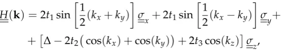
∆−2t2 cos(kx) +cos(ky)+2t3cos(kz)σ_z,

(1.13)

wheret1represents the strength of hopping between theAandBsub-lattices in the

same layer,t2represents the strength of hopping between atoms of the same species

in the same layer,t3represents the strength of hopping between atoms of the same

species in adjacent layers and ∆ represents the sub-lattice energy difference. The lattice spacing has been chosen asax = ay = az = 1. Degeneracies occur at points in reciprocal space where each component hi(k) of the Hamiltonian (1.13) vanish simultaneously. Clearly theh1(k)andh2(k)components both vanish at (kx,ky) =

(0, 0)and(kx,ky) = (π,π). The solutions ofh3(k) =0 for each of these(kx,ky)pairs leads to two equations:

cos(kz) =−

∆ 2t3

−2t2

t3

, (1.14)

cos(kz) =−

∆

2t3

+2t2

t3

. (1.15)

The values of the quantities ∆/2t3 and 2t2/t3 determine if there are solutions to

h3(k) = 0 at all . If there are solutions each of the equations contributes a pair of

[image:36.595.171.452.287.337.2]

Weyl points at±kzof opposite helicity.

Figure 1.6 shows the topological phase diagram of the Hamiltonian (1.13). There are two distinct gapped insulator phases and three Weyl semi-metal phases. The two insulator phases are a normal topologically trivial insulator and a quantum hall insulator, respectively. The three Weyl semi-metal phases represent solving either of the two equations (1.14) and (1.15) individually or both simultaneously.

We shall focus on the phase WSM1; where the two Weyl points occur at

(37)

1.4. Topological Features in Three Dimensional Dispersions 15

FIGURE 1.6: A phase diagram representing the topological phases of the Hamiltonian (1.13). The phases are displayed in the accom-panying legend. The phases NI and QHI represent normal insula-tors and quantum Hall insulainsula-tors respectively. The phases labeled WSM represent one of three different Weyl semi-metal phases. In the phase WSM1 there are two Weyl points which appear along the line kx = ky = 0. In the phase WSM2 there are two Weyl points which

appear along the linekx=ky=π. In the phase WSM3 there are four

Weyl points which appear at each of the locations of the WSM1 phase and the WSM2 phase.

occur atkz =±π/2 as shown in the figure 1.7.

The expansion of the Hamiltonian around the points(0, 0,±π/2)results in the

local behaviour:

H(k)'t1(kx+ky)σ_x+t1(kx−ky)σ_y∓2t3(kz∓ π

2)σz. (1.16) From this expansion we can determine that the charges of these two Weyl points are c = ±sgn(t3). As the ratios of ∆/2t3 and 2t2/t3 depart from unity the Weyl

points move along the linekx = ky = 0. Beyond certain critical values the Weyl points meet and annihilate, either atkz = 0 or kz = π, and we reach one of the

gapped insulator phases.

(38)

FIGURE1.7: Density plot representing the magnitude of the vector

h(k) over the three dimensional Brillouin zone. The magnitude of this vector represents half the splitting between the two bands of the band structure. The parameters have been chosen so that we are in the phase WSM1. The two Weyl points, for these parameters, occur at(0, 0,±π

2)

FIGURE1.8: A plot taken from Delplace et al. [72] showing two of the surface bands of the WSM1 phase plotted over a shifted surface Brillouin zone. In Delplace et al. [72] terminations of the bulk Hamil-tonian (1.13) in thexzplane were considered. The surface band struc-ture shows the open Fermi arc degeneracy joining the projections of the bulk Weyl points which are indicated byW− andW+. The

sur-faces are coloured according to the legend and represent the average positionhyiof the corresponding states.

1.5 Topological Features of Dissipative Systems

(39)

1.5. Topological Features of Dissipative Systems 17

combined action of the parity, P, and time reversal, T, operators. In quantum mechanics the Hamiltonian is usually assumed to be Hermitian resulting in real eigenvalues and unitary time evolution which conserves the overall probability. An interesting aspect of non-Hermitian PT symmetric Hamiltonians is that they can also display unitary time evolution and hence could describe new classes of complex quantum theories [74].

Beyond PT symmetry there is interest in systems that display dissipation and amplification more generally. In these systems the eigenvalues can be complex with unconventional consequences. Many of these curiosities are linked to the presence of exceptional points - locations in parameter space where two or more complex eigenvalues and their associated eigenvectors coalesce. These exceptional points often, but not always, occur at points in parameter space where PT symmetry is broken [75]. Initially it was believed that one such unconventional aspect is that as exceptional points are encircled once in parameter space the modes are swapped, and thus it requires twice encircling the exceptional point in order to return to the original state [76]. Even then the states have accumulated a Berry phase of

π, so it would therefore take four circuits to return fully to the original situation

[77]. Such a perspective of state-flips and geometric phases however requires the instantantaneous eigenstates to be followed upon the encircling evolution. The non-Hermitian nature of these systems however can lead to a breakdown of the adiabatic theorem [78, 79]. Recently it was shown that the effect of the breakdown of the adiabatic theorem is that the direction of encircling of the exceptional point completely determine the eigenvalue sheet which one ends up on [80]. The presence of exceptional points also gives rise to novel edge features as discussed by Leykam et al. [81]. In Leykam et al. [81] the authors discovered that there are two types of topological charges associated with exceptional points, one a generalisation of the Berry phase and a second one with no Hermitian counterpart, which in combination can produce myriad diverse edge theories.

(40)

systems to exceptional points, allowing mode selection [84], and on going through exceptional points, resulting in unconventional behaviour in laser systems [85]. Beyond marked behaviour changes achieved by traversing through exceptional points there is interest in exploiting the topological structure of the eigenvalue sheets around the exceptional points in optical systems [86].

The type of systems which exhibit exceptional points need not be especially com-plicated, in either a mathematical or physical sense. As an example we shall consider a simple model of coupled lossy modes that exhibits exceptional point physics:

H= ω1−iγ1 µ

µ ω2−iγ2

!

. (1.17)

In equation (1.17)ω1 and ω2 are two distinct mode frequencies and γ1 andγ2 are

the corresponding loss rates. The coupling strength between the modes isµ. The

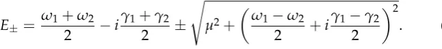
eigenvalues of this model are

E±= ω1+ω2

2 −i

γ1+γ2

2 ±

s

µ2+

ω1−ω2

2 +i

γ1−γ2

2

. (1.18)

The difference of the two eigenvalues only depends on the difference of the two mode frequencies and the differences of the two loss rates and not the average of the mode frequencies and loss rates. As such to find exceptional points we need only examine the difference in these quantities for a chosen fixed couplingµ.

FIGURE1.9: The real and imaginary parts of the eigenvalues of the Hamiltonian (1.17). For this plot we have consideredωav = 1 and

[image:40.595.162.485.345.381.2]

γav=1. The chosen coupling strength isµ=0.1.

Figure 1.9 shows the real and imaginary parts of the eigenvalues as a function of the difference in mode frequencies and difference in loss rates. We see that an exceptional point occurs at (δω,δγ) = (0, 0.1), corresponding to the difference in

loss rates matching the strength of coupling.

(41)

1.6. Iso-Frequency Surfaces 19

FIGURE1.10: The real (continuous) and imaginary (dashed) parts of the eigenvalues of the Hamiltonian (1.17) along the lineω1=ω2.

there are extended degeneracies in the real parts and in the imaginary parts of the eigenvalues. These extended degeneracies are non-overlapping except at the two exceptional points locations at δγ = ±µ = ±0.1 indicated by the black dashed

gridlines. The dispersion away from the exceptional points for both the real and imaginary parts exhibit square-root dependence, a hallmark of the lowest order exceptional point.

1.6 Iso-Frequency Surfaces

The previous sections have considered the topological classification of band structures, i.e. assigning topological invariants to the surfaces ω(k), where k is

either (effectively) a two dimensional or three dimensional wavevector. It is also possible however to characterise a different surface: the iso-frequency surface of a material. This construction is a closed surface in wavevector space representing all the wavevectors that a wave of a given frequency can propagate with. In electronic settings a well known example of one of these surfaces is the Fermi surface which is the surface of all wavevectors that can propagate at the Fermi frequency. In optical systems the analogous surface is set by the frequency of the incoming light. The iso-frequency surface is then an important descriptor of the refraction and polarisation behaviour of the material in optical contexts.

(42)

This first approach, by Gao et al. [87], studies the iso-frequency surfaces of effectively homogeneous uniaxial hyperbolic metamaterials with chirality. In this context, prior to the introduction of chirality, the iso-frequency surface has three sheets and features two isolated degeneracies between pairs of the sheets. For a chosen frequency the sheets of this surface represent the allowed wavevectors that light of a given polarisation can propagate in the uniaxial hyperbolic material with. The degeneracies of the surface are quadratic intersections rather than the linear Dirac point crossings in section 1.2. In this instance the quadratic degeneracies have a topological index of ±1 rather than the±1

2 of Dirac points. The introduction of

chirality then lifts both degeneracies resulting in non-zero Chern numbers for each sheet of the iso-frequency surface. The distinction between the topological indices of linear and quadratic degeneracies can have global consequences on the allowable Chern numbers of the surfaces, as we shall later explore.

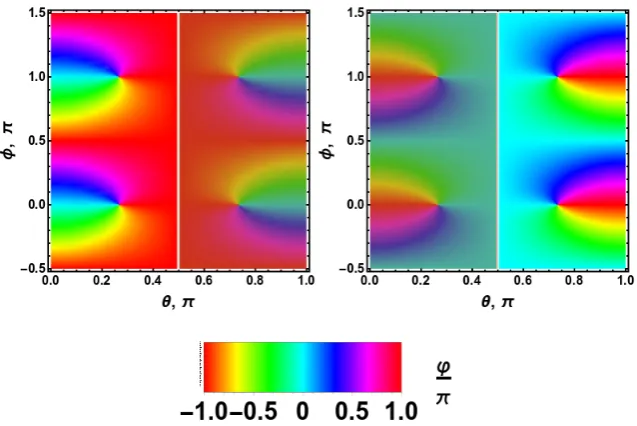
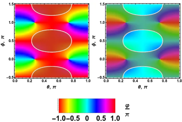
It is worth examining the work of Gao et al. [87] in relation to the Chern insulator model presented in section 1.3. One difference is in the work of Gao et al. [87] the relevant reciprocal space is not the Brillouin zone torus but rather the sphere of propagation directions. This is a noteworthy distinction as in the work of Gao et al. [87] the degeneracies are not generated by lattice effects but rather by the anisotropy of the optical material. A second difference is that the authors here are considering the polarisation texture in reciprocal space [89] as generating the topologically non-trivial result rather than some complicated orbital hybridisation behaviour in reciprocal space. In this context the Dirac points and zeroes of the mass terms, discussed in section 1.3, are then polarisation features known as C-points and L-lines [90, 91]. C-points are directions in reciprocal space where the polarisation state is purely circularly polarised, either left-handed or right-handed. L-lines are directions in reciprocal space along which the polarisation state is linear. In the language of polarisation optics a non-zero Chern number results from the L-lines separating C-points of different handedness [89].

(43)

1.7. Light-Matter Coupling in Semiconductors & Topological Polaritons 21

subsection 1.3.3. In particular, a triangular geometry was considered in Rechtsman et al. [88] so as to produce Dirac point degeneracies in the bandstructure and a perturbation, the effective external field induced by the helical waveguides, lifts the degeneracies producing a topologically non-trivial result.

Although not explicitly stated, focusing on these Floquet “quasi-energies” is similar to analysing iso-frequency surfaces of photonic crystals. Rechtsman et al. [88] are looking at the form of the quasi-invariants which evolve the field along the structure. The “quasi-energy” surface is in fact a closed surface in wavevector space meaning that the surface is more accurately described as a quasi iso-frequency sur-face. The Floquet quasi-invariants are therefore similar to the iso-frequency surface if one thinks of the latter as a surface ofkz(kx,ky). In the work of Rechtsman et al. [88] a scalar wave equation was employed, implicit in which is an assumption that the polarisation state is completely decoupled from the direction of propagation. This assumption is generally not the case; for instance polarisation mixing occurs for light propagating in anisotropic materials.

In this thesis we shall present work which is complementary to these two diverse realisations of optical topological order. As in the work of Gao et al. [87] we will eschew the reliance on a particular form of lattice patterning to produce de-generacies and instead rely on the intrinsic polarisation dede-generacies of anisotropic dielectrics. We will consider both homogeneous materials, as was done in Gao et al. [87], and periodic structures. In the former instance the distinction between our work and that of Gao et al. [87] is that we will consider several different forms of biaxial anisotropy rather than uniaxial anisotropy. In the latter case the distinction, as well as considering more general anisotropic materials, is that the topology of the Brillouin zone torus differs compared to the sphere of propagation directions. Such a difference in topology will require a different polarisation texture in reciprocal space and will therefore have a different topological phase diagram to that of the homogeneous material. The work we present will be complementary to that of Rechtsman et al. [88] in the sense that we will also consider light propagating out of the periodic plane of a two dimensional photonic crystal. The distinction for us is that we will exploit the effective optical spin-orbit coupling of anisotropic materials rather than considering the decoupling of the polarisation and the direction of propagation in reciprocal space.

1.7 Light-Matter Coupling in Semiconductors & Topological

Polaritons

(44)

appropriated by many other diverse settings. In the previous sections we primarily focused on the relevance of topological concepts to optical systems as that shall be one of the two primary settings of the work presented in this thesis. The other setting we shall be considering is that of exciton-polariton systems.

An exciton is an elementary excitation of a semiconductor. This excitation comprises a valence band hole and a conduction band electron which are bound by their Coulomb attraction [17]. There are in fact a number of discrete exciton energy levels just below the semiconductor band-gap as well as the continuum of unbound yet interacting electron and holes above the electronic band-gap [92]. For light impinging upon a semiconductor, with a frequency just below that of the band-gap frequency, the excitons make a significant contribution to the optical response of the material [93]. The effect of the excitons is to heavily modify the linear photonic dispersion resulting in mixed light-matter modes known as polaritons [17].

These polaritons have proved an interesting platform to study myriad phenom-ena. In particular microcavity polaritons resulting from the coupling of heavy-hole quantum-well excitons to photonic cavity modes have allowed polariton condensa-tion [94] and consequently polariton lasing [95], among many other effects. Within the microcavity polariton setting there has also been several proposals [34–36] and a realisation [96] of various topological insulators in two dimensions characterised by non-zero Chern numbers. These schemes have considered the implementation of triangular two dimensional lattice potentials for either the excitonic [34, 36] or the photonic component [35] of the polaritons so as to produce Dirac point in the polaritonic band-structure. The degeneracies at the Dirac points were then lifted due to the Zeeman splitting of the bright excitons arising from the introduction of a magnetic field. The result of this is to achieve the desired set of topologically non-trivial bands.

(45)

1.8. Outline of Thesis 23

1.8 Outline of Thesis

In this thesis we consider the topological characteristics, both in terms of topological invariants and topologically protected degeneracies, of various photonic systems. This work leads to new theoretical understanding of the topological characteristics of bulk homogeneous dielectrics, patterned two dimensional photonic crystals and bulk magneto-exciton-polaritons.

In chapter 2 we examine the topological invariants that can be assigned to the refractive index surfaces of anisotropic optically active bulk dielectric media. We examine specifically the L-lines and C-points for light propagating through biaxial dielectrics and how these polarisation degeneracies can lead to non-zero Chern numbers once gyromagnetic effects are introduced. In this chapter we also derive an effective Hamiltonian which paraxially evolves the field along one of the optic axis directions of the biaxial dielectric.

In chapters 3 and 4 we make use of the Hamiltonian derived in chapter 2, adapting it to describe light propagating through two dimensional photonic crystals with two different lattice geometries. In chapter 3 we consider square patterned photonic crystals while in chapter 4 we consider triangularly patterned photonic crystals. In each chapter we determine the Chern number of the iso-frequency surface for crystals primarily composed of biaxial materials with one of two possible forms of optical activity. For all combinations of form of lattice and optical activity we examine the topological phase diagrams. We compare the topological phase diagrams achieved in each geometry and contrast them with those of the homogeneous materials considered in chapter 2.

In chapter 5 we examine the bulk-boundary correspondence of topologically non-trivial materials. We investigate this correspondence for two different bound-ary conditions; one of which explicitly includes the adjacent material. For each type of boundary condition we explore the fate of the edge states as the bulk band gap is closed. We also explore the role that the orientation of the boundary plays in the emergence of edge states. Using these insights we address the question of edge states for the bulk photonic crystal models developed in the previous chapters.

(46)

(47)

25

Chapter 2

Propagation of Light Through

Anisotropic Optically Active

Materials

2.1 Introduction

In this chapter we study the propagation of light through homogeneous anisotropic materials which additionally exhibit gyrotropic effects. The anisotropy we consider is that of an optically biaxial crystal resulting from low crystal symmetry [13]. In these materials double refraction is the norm, with the two refractive indices as well as the natural polarisation state of the light varying with the direction of propagation through the material [97]. These refractive indices coalesce and come apart four times over all possible propagation directions. These points of contact in direction space are the conical intersections of the refractive index surfaces and shall be of primary interest in this chapter.

We shall see that the introduction of optical activity can cause these conical intersections to disappear resulting in two distinct refractive indices for light travelling in any direction [14]. With this addition the polarisation state is in general that of elliptic polarisation, with departures from this general state worthy of attention. These departures are in the form of either C-points or L-lines, the former being points in direction space at which the polarisation is circular and the latter being contours in direction space along which the polarisation is linear [91].