Applied Mathematics, 2014, 5, 3156-3205
Published Online November 2014 in SciRes. http://www.scirp.org/journal/am http://dx.doi.org/10.4236/am.2014.519298
Modeling the Dynamics of Malaria
Transmission with Bed Net
Protection Perspective
Jean Claude Kamgang1, Vivient Corneille Kamla1, Stéphane Yanick Tchoumi2
1Department of Mathematics and Computer Sciences, ENSAI, University of N’Gaoundéré, N’Gaoundéré,
Cameroon
2Department of Mathematics and Computer Sciences, Faculty of Science, University of N’Gaoundéré,
N’Gaoundéré, Cameroon
Email: [email protected], [email protected], [email protected]
Received 11 September 2014; revised 15 October 2014; accepted 29 October 2014
Copyright © 2014 by authors and Scientific Research Publishing Inc.
This work is licensed under the Creative Commons Attribution International License (CC BY). http://creativecommons.org/licenses/by/4.0/
Abstract
We propose and analyze an epidemiological model to evaluate the effectiveness of bed nets as a prophylactic measure in malaria-endemic areas. The main purpose in this work is the modeling of the aggressiveness of anopheles mosquitoes relative to the way humans use to protect themselves against bites of mosquitoes. This model is a system of several differential equations: the number of equations depends on the particular assumptions of the model. We compute the basic re- production number 0, and show that if 0≤1, the disease free equilibrium (DFE) is globally asymptotically stable on the non-negative orthant. If 0 > 1, the system admits a unique endemic equilibrium (EE) that is globally and asymptotically stable. Numerical simulations are presented corresponding to scenarios typical of malaria-endemic areas, based on data collected in the literature. Finally, we discuss the relative effectiveness of different kinds of bed nets.
Keywords
Epidemiological Model, Malaria, Basic Reproduction Number, Lyapunov Function, Global Asymptotic Stability, Non-Standard Finite Difference Scheme (NFDS), Simulation
1. Introduction
Asia and much of Africa. Humans contract malaria following effective bites of infected Anopheles female mos-quitoes during blood feeding. Plasmodium falciparum is the most common cause of malaria mortality in Africa, and the chain of transmission can be broken through the use of insecticide-treated bed nets and anti-malarial drugs, as well as other control strategies.
Malaria accounts for more than 207 million infections and results in over 627,000 deaths globally in 2012 [1]. About 90% of these fatalities occur in Sub-Saharan Africa [1] [2]. Despite intensive social and medical research and numerous programs to combat malaria, the incidence of malaria across the African continent remains high.
In the field of mathematical epidemiology, numerous models have been proposed with the purpose of under- standing various aspects of the disease. The foundation model of Sir Ronald Ross, originally proposed in 1911
[3] and extended by MacDonald in 1957 [4], serves as the basis for many mathematical investigations into the epidemiology of malaria. A prominent example is the model of Ngwa and Shu [5], which introduces susceptible (S), exposed (E), and infectious (I) classes for both humans and mosquitoes, plus an additional Immune class (R) for humans. This model is extended in the Ph.D. theses of Chitnis [6] and Zongo [7] (these two theses also pro-vide comprehensive reviews on the state of the art). Chitnis introduces immigration into the host population, which is a significant effect since hosts migrating from a naive region to a region with high endemicity are espe-cially susceptible to infection. Zongo further extends the model by dividing the human population into non- immune and semi-immune sub-populations, which are modeled using (SEIS) and (SEIRS) model types, respec-tively.
In his thesis, Chitnis espoused the use of insecticide-treated bed nets, coupled with rapid medical treatment of new cases of infection, as the best strategy to combat malaria transmission. In this paper we make further exten-sions to the model to include the effects of bed-net use on malaria transmission. In particular, we divide the hu-man population into groups that are characterized by the methods they use to protect themselves against the mosquito bites. These assumptions are consistent with the observable situation in many endemic areas, parti- cularly in poor countries. We believe that the current study represents the first systematic model-based analysis of the impact of bed nets on the dynamics of malaria transmission.
Malaria is highly seasonal [8] [9]: the highest endemicity typically occurs during rainy seasons, when mos-quito density is high due to high humidity and the presence of standing water where mosmos-quitoes can breed. Dur-ing this period, even people with immune predisposition to malaria infection are at risk of attainDur-ing the critical level of malaria parasites in their bloodstream that could make them fall sick. In our model, we consider condi-tions characteristic of a rainy season in a region of high malaria endemicity: typically, such condicondi-tions last for a period between three to six months. Because of the brevity of the period being considered, we neglect the effects of death, birth and migration of hosts. We also omit exposed and recovered classes for hosts: due to the high density of anopheles mosquitoes during such periods, exposed individuals rapidly become infectious, and the partial immunity of hosts following recovery has negligible effect. Results for more sophisticated models that include exposed and/or recovered state(s) are reserved for forthcoming papers.
The paper is organized as follows. Section 2 describes our model and gives the corresponding system of dif-ferential equations. Section 3 establishes the well-posedness of the model by demonstrating invariance of the set of non-negative states, as well as boundedness properties of the solution. The equilibriums of the system are calculated, and a threshold condition for the stability of the disease free equilibrium (DFE) is calculated, which is based on the basic reproduction number 0. The method used to derive the basic reproduction number is different for the method of the next generation operator of Van Den Driesshe and Watmough [10] currently used in literature. Section 4 analyzes the stability of equilibriums. We prove in Section 4.1 the global asymptotic sta-bility (GAS) of the disease free equilibrium (DFE) when 0 ≤1; in Section 4.2 we prove the GAS of the en-demic equilibrium (EE) when 0 >1. Section 5 provides graphs of trajectories corresponding to various para-meter sets computed based on data obtained from the literature. Section 6 discusses the significance of our re-sults. Finally, the Appendix contains detailed proofs and computations required by the analysis.
2. Model Description and Mathematical Specification
J. C. Kamgang et al.
2.1. Host Population Structure and Dynamics
The human population is divided into n+1 groups. One of these groups consists of humans who do not use bed nets, while the other n groups correspond to the various types of bed nets used as protection against mos-quito bites. Some nets are untreated; others are treated with repellent; others are treated with insecticides, with varying degrees of toxicity (toxicity typically decreases with use). We let b ii 1,
(
= ,n)
denote the proportion of the human population that is in the ith protected group, and 01 1
n
i i
b b
=
≡ −
∑
is the proportion of humans that use no protection.The dynamics of the th
i host population
(
i=0,,n)
is described by a SIS-based compartment model as shown in Figure 1. As explained in the Introduction, we omit exposed and recovered classes, as well as the ef- fects of birth, death, and migration. The incidence of infection for humans in the thi group is given by i q I am
H ,
where a is the average number of bites per mosquito per unit time (the entomological inoculation rate); Iq is the number of infectious mosquitoes; H is the human population; and mi is the infectivity of the mosquito within the contact with human of the ith group, that is the probability that the bites of an infected mosquito on a susceptible human of the ith group will transfer infection to the bitten human.
2.2. Mosquito Population Structure and Dynamics
The population of disease vectors (adult female anopheles mosquitoes) is characterized by several classes, where each mosquito’s class membership is determined by its own history of past activity. Newly-emerged adult mos-quitoes initially enter the susceptible class: the rate of entry (that is, the recruitment rate) is Γ. Also included within the susceptible class are all uninfected mosquitoes: this includes mosquitoes that have never fed, as well as those that have fed but have never become infected. This is a reasonable approximation, since all such mos-quitoes are in the same state with respect to progress of the infection. The natural death rate for mosmos-quitoes (apart from mortality due to being killed while feeding) is µ.
Adult mosquitoes alternate between two activities: questing (that is, seeking a host to bite for its blood meal)
and resting (to lay down eggs, or to digest a blood meal). In the current model we assume that all susceptible
mosquitoes are in the questing state: the presence of susceptible resting mosquitoes can be approximately ac-commodated by reducing Γ to account for recruited mosquitoes that are resting and not questing. We are cur-rently working on an improved model that explicitly includes the class of susceptible resting mosquitoes.
Questing mosquitoes are equally likely to feed on any human, regardless of his/her protection method. Thus for any given blood meal, the probability that the human host belongs to the ith group is bi. During a blood meal on a human in the ith group, the mosquito is killed with probability ki, survives with probability ki ≡ −1 ki, and succeeds in feeding with probability k fi i. Letting a denote the average number of bites per mosquito per unit time (the entomological inoculation rate) it follows that the incidence rate of successful blood meals is
0 n
i i i i
ab f k ϖ
=
≡
∑
, while the additive death rate caused by the questing activity of mosquitoes is 0 ni i i
d ab k
=
≡
∑
. If we let Ii and Ii denote respectively the number of infected humans in group i and the probability that the bite of a mosquito on humans in group i will infect the mosquito, then the incidence rate for mosquitoes be- coming infected is0 n
i i i i i
I ac f k
H ϕ
=
≡
∑
.Susceptible mosquitoes that become infected enter the first exposed resting class
( )
Er( )1 . Following initial infection, the mosquito must remain alive for a certain period before becoming infectious. This period is known in biological and medical literature as extrinsic incubation period [11]. During this period, the mosquito expe-riences a certain number of periods of questing and resting. In our model, we suppose that a mosquito becomesinfectious after a fixed number l of resting/questing cycles following initial infection. These successive resting/ questing cycles are modeled as a sequence of 2l exposed states, and are denoted by Eq( )1, , , , Er( )2 Eq( )l Er( )l1
+
.
If a mosquito survives through all of these state, it then enters the infectious class, which is further divided into questing and resting sub-classes (Iq and Ir, respectively). Once a mosquito enters the infectious class, it re-mains there for the rest of its life, alternating between questing and resting states.
The overall dynamics of the mosquito population is depicted in the multi compartment diagram in Figure 2: The fundamental model parameters are summarized in Table 1, while derived parameters are summarized in
Table 2.
Γ
q q
μ μ
μ
μ μ
μ
q q
r r
r
Figure 2. Mosquito population dynamics.
Table 1.Fundamental model parameters.
Param. Description
a Biting rate of the vectors.
i
b Proportion of th
i host group.
i
c Infectivity coefficient of vector due to bite of th
i host group.
i
f Probability that a vector which bites the th
i host group and survives obtains a blood meal.
i
k Probability that a vector attempting to bite th
i host group is killed.
i
m Infectivity coefficient of hosts in th
i group due to bite of infectious vector.
δ Rate at which resting vectors move to the questing state.
i
γ Transition rate from infectious to susceptible states for hosts in the th
i group. µ Natural death rate of vectors.
Table 2. Derived model parameters.
Param. Formula Description
d
0
n ii i
ab k
=
∑
Death rate of vectors due to questing activity.q f
ˆ
ϖ
µ ϖ+ Frequency for questing mosquitoes.
r
f µ δδ
+ Frequency for resting mosquitoes.
i
k 1−ki Survival probability of vectors attempting to bite
th
i host group.
ˆ
µ µ+d Death rate of questing vectors. ϕ
0
n i i i i i
I ac f k
H
=
∑
Incidence rate of infection for questing susceptible vectors.ϕ
0
n i i ii i
ac f k b
=
∑
Maximum incidence rate of infection for questing susceptible vectors.ϖ
0
n i i i i
ab f k
=
J. C. Kamgang et al.
2.3. Model Equations
The system of ordinary differential equations that characterize the model are given as follows:
(
)
( )(
)
( ) ( ) ( )(
)
( ) ( ) ( )(
)
( )(
)
( )(
)
(
)
1 1 1 1 1 ˆˆ 1, 2, ,
1, 2, ,
0,1, ,
ˆ
q q
r q r
j j j
q r q
j j j
r q r
q
i i i i i i
l
q r q r
r q r
S S
E S E
E E E j l
E E E j l
I
I am Hb I I i n
H
I E I I
I I I
µ ϕ
ϕ µ δ
δ µ ϖ
ϖ µ δ
γ
δ µ ϖ δ
ϖ µ δ
+ +
+
= Γ − +
= − + = − + = = − + = = − − = = − + + = − + (1)
The system (1) together with initial conditions completely specifies the evolution of the multi-compartment system shown in Figure 1 and Figure 2. Note that system (1) also determines Si (susceptible hosts of the
th i hosts group, since each host sub population is closed and Si =Hbi−Ii.
3. Well-Posedness, Dissipativity and Equilibria of the System
In this section we demonstrate well-posedness of the model by demonstrating invariance of the set of non- negative states, as well as boundedness properties of the solution. We also calculate the equilibriums of the system, whose stability properties will be examined in the following section.
3.1. Positive Invariance of the Non-Negative Cone in State Space The system (1) can be rewritten in matrix form as
( )
( )
(
( )
)
( )
ˆ ( ) ˆ ˆ ˆ q q q qI I I
I I I
S S
S µ ϕ S = − +µ ϕ −µΓ−ϕµΓ
= − + + Γ
= + ⇔ ⇔ = =
x A x x b x
x A x x
x A x x
(2)
Equation (2) is defined for values of the state variable x=
(
Sq;xI)
lying in the non-negative cone of u(
u= + +n 2l 4)
, which we denote as u+. Here xS ≡Sq represents the naive vector component, and ( ) ( )(
)
( )( )
(
1)
0 1
; ; ; ; ;
j j l
I Er Eq j l Er Ii i n I Iq r
+
≤ ≤ ≤ ≤
≡ x
represents the non-naive components of the state of the system. This notation is consistent with the notation of reference ([12]), and we use results from this reference in our analysis.
The matrix AI
( )
x may be written in block form as( )
( )
( )
,( )
( )
,E I E
E I I
I I I I I =
A x A x
A x
A x A x (3) where the four matrices blocks may be described as follows:
The
(
2l+ ×1) (
2l+1)
matrix AIE( )
x expresses the interaction between non-infected components of the system. It is a 2-banded matrix whose diagonal and sub-diagonal elements are given by the vectors d0 and d−1 respectively, defined by(
) (
)
(
) (
) (
)
0 1
2 components 2 components
ˆ ˆ
, , , , , ; , , , ,
l l
µ δ µ ϖ µ δ µ ϖ µ δ − δ ϖ δ ϖ
= − + − + − + − + − + =
d d (4)
The
(
2l+ × +1) (
n 3)
matrix AII E,( )
x gives the dependence of the exposed components( ) ( )
the infected components
(
I ii(
=0,,n)
,I Ir, q)
. The only nonzero entries in this matrix are the first n+1 terms of the first row, which are given by ac f ki i iSq, 0,i ,nH = : these terms characterize the transition of
vectors from the susceptible to the first exposed state, which depends on infectious the host components. The
(
n+ ×3) (
2l+1)
matrix AIE I,( )
x gives the dependence of infectious components on exposed components. All entries are zero except the(
n+2, 2l+1)
entry, which is equal to δ reflecting the transition rate of vectors from state Er( )l 1+
to state Iq.
The
(
n+ × +3) (
n 3)
matrix( )
I IA x may be written in block form as
( )
( )
( )
,Ih Iv h I Iv I I I I =
0
A x A
A x
A x , with
( )
0 diag
Ih
q
I i i
i n I
am
H γ ≤ ≤
= − −
A x ;
( )
(
ˆ)
(
)
Iv I
µ ϖ δ
ϖ µ δ
− +
= − +
A x ; ,
0 0 0
0 Ivh
I n n b am b am = A .
Remark 3.1. The second matrix form given in (2) can also be written in the form
( )
(
)
( )
,
,
S S S S S I I
I I I
∗ = − + =
x A x x x A x
x A x x
(5)
where AS
( )
x = − −µ ϕˆ , , 0 0 0 2 1 entries0, 0, , 0 , , , , 0, 0 ˆ
S I n n n
l a
f c k f c k
H µ + Γ =
A , and
ˆ
S µ
∗ = Γ
x is the component of the DFE (see Proposition 3.5 below) in the disease free sub-variety For such a system, Kamgang et al. in [12]
gives a threshold condition for the stability of the DFE and an analysis of global asymptotic stability that we may apply to the current system.
For a given x∈u+, the matrices A x
( )
, AS( )
x and AI( )
x are Metzler matrices. The following proposition establishes that system (2) is epidemiologically well posed.Proposition 3.1. The non-negative cone u+ is positively invariant for the system (2).
Proof. For any x∈u+, the matrix A x
( )
is a Metzler matrix (see Appendix); and it is well-known thatsystems determined by Metzler matrices preserve invariance of the non-negative cone. □ 3.2. Boundedness and Dissipativity of the Trajectories
We have the following proposition.
Proposition 3.2. The simplex
(
, 0)
ˆ ˆ
u
q i i I
x S I Hb i n M ϕ
µ µ µ
+
Γ Γ
Ω = ∈ ≤ ∧ ≤ ≤ ≤ ∧ ≤
(6)
where
(
( ) ( ))
( )1 1l
j j l
I q r r q r
j
M E E E + I I
=
≡
∑
+ + + + and0 n
i i i i i
a c b f k
ϕ
=
≡
∑
is a compact forward-invariant and absorb-ing set for the system (1).
Note that MI is the overall population of non-naive mosquitoes; while ϕ is the maximum incidence rate of infection for questing susceptible mosquitoes.
Proof. From (1) we have Sq= Γ −µˆSq−ϕSq as dynamic of susceptible mosquitoes; thus Sq ≤ Γ −µˆSq. It
follows that limsup
( )
ˆ q t S t µ →+∞ Γ= . From (1) we also have i i q
(
i i)
II am Hb I
H
≤ −
, i=0,,n, so similarly
( )
limsup i i
t
I t Hb
→+∞ ≤ . Finally, by adding together the equations for exposed and infectious vector populations in system (1) we obtain MI ≤ϕSq−µMI; and since
ˆ q S
µ Γ ≤ and
0 0
n n
i i
i i i i i i
i i
I H
a c f k a c f k
H H
ϕ ϕ
= =
=
∑
≤∑
= we ob-tain
ˆ
M ϕ µM
µ Γ
≤ −
. It follows that limsup
( )
ˆ It
M t ϕ
µ µ
→+∞
Γ
J. C. Kamgang et al.
As a result of Proposition 2, we may limit our study to the simplex specified in (6). 3.3. Computation of the Threshold Condition
Several techniques exist for computing the basic reproduction number and threshold conditions for the local asymptotic stability of the disease free equilibrium of epidemiological models represented by systems of ordi-nary differential equations. In [10] the maximum eigenvalue of next generation operator is proposed. In many other papers in the literature, either the technique in [10], or the Routh-Hurwitz criterion are used [13]-[15]. Unfortunately, these are not suitable for large-scale systems that may possess many equations. Instead, we use the technique in [12] to compute the threshold condition for the system under consideration, which also enables the evaluation of the basic reproduction number. Specifically, we have:
Proposition 3.3 ([12]). Let M be a Metzler matrix with block decomposition =
A B
M
C D where A and
D are square matrices. Then M is Metzler stable if and only if A and − −1
D CA B (or D and − −1
A BD C)
are Metzler stable.
We refer the reader to reference [12] for the proof of the proposition. This result enables the reduction of the large-scale matrix M to a number of smaller-scale matrices, to which more classical methods may be applied.
Proposition 3.4. The basic reproduction number for the system (1) is
( )
(
)
1 2 0 =0 ˆ 1 l nq r i i i i i
i i
q r
f f a b c f k m
H
f f µ γ
ϖ
+
Γ ≡
−
∑
(7)
where ˆ q f ϖ µ ϖ ≡
+ and fr δ µ δ
≡
+ are respectively the questing and the resting frequencies of mosquitoes.
The proof of the above proposition is postponed to Appendix B. 3.4. System Equilibria
Steady states of the system are specified by the following proposition.
Proposition 3.5. System (2) admits two equilibriums. The first (called the disease free equilibrium or DFE) is
given by x∈u+, where
(
Sq; I)
u∗ ∗ ∗
+
= ∈
x x with I u1
∗= ∈ −
0
x and
ˆ q S
µ
∗=Γ
. The second (called the en-
demic equilibrium or EE) is given by
(
)
(
)
(
)
( ) ( )(
)
( )(
)
(
)
(
)
1 1 1 1 1 1 , , ˆ ˆ 1 1, , 1 ,
, 0 .
r q q l q r
q l r q r q r q
q q r
q r q r
j j
q l j q r l j q
q r q q r
i i q i
i i i q
f f I f f
S I I f I E I
f f f
f f f f
E I E d I j l
f f f f f
ab m I
I H i n
H ab m I
ϖ ϖ ϖ ϖ
µ µ µ δ δ δ
ϖ δ γ + + + − + − − − Γ = − = = = + − − = = ≤ ≤ = ≤ ≤ + (8)
where
(
)
1 0, 1 l q r q q r f f I f f ϖ +
Γ
∈
−
is the finite root of the equation
(
)
(
)
(
)
2 1 0 ˆ 1 1 n r q i i i i il
i i i
q r r q
f f b m c f k
a
H am x f f f f x
µϖ
γ + ϖ
=
− =
+ Γ − −
∑
(9)The proof of Proposition 3.5 is postponed to Appendix C.
, r q
f f , and l) as well as the protection means used by the population (expressed in the parameter ϖ )
strongly influence the location of the EE. This justifies our assertion that mosquito dynamics and host protection means are important practical factors in determining the prevalence of infection.
4. Stability of System Equilibria
In this section we analyze the stability of the system equilibriums given in Proposition 3.5. 4.1. Global Asymptotic Stability of the Disease Free Equilibrium (DFE) We have the following result for the global asymptotic stability of the disease free equilibrium:
Theorem 4.1. When 0≤1, then the DFE for system (2) is GAS in u
+
.
Proof. Our proof is based on Theorem 4.3 of [12], which establishes global asymptotic stability for
epidemi-ological systems that can be expressed in the matrix form (5). This theorem is restated as Theorem A.1 in the Appendix: for the proof, the reader may consult [12]. To complete the proof, we need only establish for the sys-tem (2) that the five conditions (h1)-(h5) required in Theorem A.1 are satisfied when 0≤1.
(h1) This condition is satisfied for the system (2) as a result of Proposition 2.
(h2) We note first that nS =1, and the canonical projection of Ω on + is 0,
ˆ
µ
Γ
=
; the system (2) re-
duced to this sub variety is Sq = Γ −µˆSq, which is obviously GAS at Sq
∗
on + and thus on since
q
S∗∈;
(h3) We consider first the case l=1 and n=1. In this case, the matrix AI
( )
x in the system (2) is( )
(
)
(
)
(
)
(
)
(
)
0 0 0 1 1 1
0 0 0
1 1 1
0 0 0 0
ˆ 0 0 0 0 0
0 0 0 0 0
.
0 0 0 0 0
0 0 0 0 0
ˆ
0 0 0 0
0 0 0 0 0
q q
I
a a
c f k S c f k S
H H
am b am b
µ δ
δ µ ϖ
ϖ µ δ
γ
γ
δ µ ϖ δ
ϖ µ δ
− +
− +
− +
= −
−
− +
− +
A x
In this case, the two properties required for condition (h3) follow immediately: off-diagonal terms of the ma-trix AI
( )
x are non-positive; and Figure 3 shows the associated direct graph G A(
I( )
x)
, which is evidently connected, thus establishing irreducibility. For general l and n the proof of (h3) is similar.(h4) Defining AI ≡AI
( )
x∗ , we have AI( )
x ≤AI ∀ ∈ Ωx , and(
{ }
)
∗+
∈ × 0 ∩ Ω
x ; thus the upper
bound of M is attained at the DFE which is a point on the boundary of Ω, and condition (h4) is satisfied. (h5) We first observe that AI is the block matrix of the Jacobian matrix of the system (1) corresponding to the infected sub-manifold, taken at the DFE. As has been pointed in [12], the condition α
( )
AI ≤1, which is equivalent to the condition that AI is a stable Metzler matrix, is also equivalent to the condition 0≤1. This fact is developed in the proof of Proposition 3.4 (see Appendix) where we compute the value of 0 by ex- pressing the stability of the Metzler matrix AI.J. C. Kamgang et al.
Since the five conditions for Theorem 4.3 of [12] are satisfied, the theorem follows. □
4.2. Stability Analysis of Endemic Equilibrium (EE)
In this section we address the analysis of the behavior of the system when the condition 0>1 holds. It is obvious that in this case the DFE is not a stable steady state of the system (1); and as stated in Proposition 3.5, the system (1) admits a unique nontrivial biologically feasible equilibrium (the EE). In the remainder of this subsection, we establish the global asymptotic stability of the EE.
Theorem 4.2. When 0>1, the EE
x of the system (1) defined in Equation (8) is GAS on
(
0)
u >
.
Remark 4.1. The above theorem implies the GAS of the EE in the non-negative cone u+, since the positive
cone
(
0)
u >
is absorbing for the system (1).
Proof. Considering the system (1) when 0>1, there is a unique EE
x with respective components given as in (8). As it is usual in the study of the stability of EE of epidemiological system in the literature [16]-[28], let
ee
V be the function defined on
(
0)
u > as follows:
( )
(
)
( )
(
( ) ( ) ( ))
( )
(
( ) ( ) ( ))
( )
(
) (
)
(
)
1 1 =1 =1 =0 1ln ln ln
1 1
ln ln ln .
l l
q
i i i i i i
ee q q q i r r r i q q q
i i
r q r q
n
q q q r r r j j j j
l
j r
r q
f
V S S S E E E E E E
f f f f
I I I I I I I I I
f f f υ + − = − + − + − + − + − + −
∑
∑
∑
x
(10)
where the coefficients, υj for j=0,1,,n, are positive constants to be determined such that the derivative of ee
V along the trajectories of the system (1) is non-positive. The technique adopted in the determination of the j
υ is that of Guo et al.[16] [17] using graph-theoretic approach to determine the global Lyapunov function for the global asymptotic stability of the EE in models involving multi-group. In their models and examples, the dynamic in divers sub-group were describe in the same shape. here is a case where it appears that this technique works also when the shape or sub-group involved in the dynamic can be different.
With these positive constants, Vee is
∞
positive definite function on
(
>0)
u; its derivative along the trajectories of the system (1) is:( )
(
)
(
(
)
)
( ) ( ) ( ) ( )( )
( ) ( ) ( ) ( )( )
( ) ( ) ( )( )
1 1 (1) 1 1 1 1 1 1 1 d ˆ1 1 1
d
1
j j
r q j
l
ee q r q q
q q r j j
j
q r r r r q q
l
j j
r q r
q r j
l
q
r r
j j
j r
r q r r q
E E
V t S E f E
S S E
t S E f f f f E
E I I
E E
f
f E
E
f f f f f
ϖ δ
δ
µ ϕ ϕ
ϖ
δ δ δ
ϖ − = + + + + = −
= − Γ − + + − − + −
− + − + − +
∑
∑
x
( )
0 1 1 1 . q rq r r
l l
q r q r
n
i
i i i q i i q i i
i i
I I
I f I
I f f I
I a
am b I m I I I
I H δ ϖ υ γ = − − + − + − − −
∑
Substituting the value of Γ, i.e. Γ =µˆSq +ϕ Sq
, after some algebraic manipulations, the above becomes:
( )
(
)
( ) ( ) ( ) ( )( )
( ) ( ) ( ) ( ) ( )( )
( ) ( ) ( ) ( ) 1 1 1 1 1 1 1 1 dˆ 2 1
d
1 1
ee q q q r r
q q q q
q q q r r
j j j
j j j
l l
q q q
r r r
j j j j j j
j q r j q r
r r q r q
V t S S S E E
S S S S
t S S S E f
E E E
E E E
E E E E
f f f f f
δ
µ ϕ ϕ ϕ
ϖ
δ + +
+ = = = − − + − + − + + − + −
∑
∑
x
( )
( )
( )
(
)
(
)
( )
1 1 0 1 2 . l r qq q q
r r r r
q q
l l l
q q r q r
r r q r q r r q
n
i
i i i i i i i q i i q i i q i i q
i i
f f
I I I
E I I I
I I
I I I I I
f f f f f f f f
I
a a
I I am b I m I I am b I m I I
H I H
ϖ
δ δ
υ γ γ
Using relations between values of components of the state of the model at the EE given in Equation (8) (see Proposition 3.5) specifically
( ) ( )
( )
( )( )
(
)
( )
( )( )
( )( )
1 2 1 1
1 1
and
i
l i
q r q q
r r r r
q l l i i
r r q r r q r q r r q r q r
f f I E
E E E E
S
f f f f f f f f f f f f f f
ϖ ϖ
δ δ δ δ
ϕ = = == + = − + + =
and after few algebraic arrangements, the above becomes:
( )
(
)
( ) ( )(
)
( ) ( ) ( ) ( ) ( ) ( ) ( ) ( ) ( ) ( ) 1 1 1 1 1 1 1 dˆ 2 2
d
2 3
ee q q r r q r q r
q q q l
q q r r r q q r q r
j j j j l
l
q q r q r r q q
q j j j j l
j
q q r q r r q q
V t S S E I I I I I
S S S
t S S E f f f I I I I
S E E E E E I I
S l
S E E E E E I I
δ
µ ϕ ϕ
ϕ ++ ++
= = − − + − + − − + + − − + − −
∑
x 0 2 . n q qi i i i
i i i i i i q i j i q
i q q i i i
I I
I I a I I
I I am I b m I I
H I I I H I I
υ γ γ
= + − + − − + − −
∑
Taking i i i q i
i
S f c k a H υ γ =
; with this values of υi we have 0 n
i i i q
i
I S
υ γ ϕ
=
=
∑
; exploiting for i=0,1,,n
identities i
i i i q i
I
I am I b
H
γ = −
, the above becomes
( )
(
)
(
)
(
)
( )( ) ( )( ) (( )) ( )( ) ( ) 0 1 1 1 1 0 1 d dˆ 2 2 2
2 2
ee
n
q q r q r q r i i
q l q i i i
i
q q q r q r i i
r r q
j j j i
n l
q i q r q r q r
i i i j j j
i q i q r j q r q r
V t
t
S S I I I I I a I I
S I m I
S S f f f I I I I H I I
S I S E E E E E
I l
S I S E E E E E
δ µ υ υ γ = + + = = = − − + − − + − − + + − − − +
∑
∑
∑
x ( ) ( ) ( )(
)
1 1 0 0 ˆ : . lq q i
r
i l
q q i
r
n n
q
q l r i i i i i i i i
i i
s r q
I I I
E
I I I
E I
S A I B a m I C I D
H
f f f
δ
µ υ υ γ
+ + = = − − = + +
∑
+∑
(11)The terms A, B, for each i, Ci and Di are non-positives by the Corollary A.1 of the Lemma A.1 (of arithmetic-geometric means inequality). A is null whenever Sq =Sq
holds; for each i, Ci is null whenever Ii=Ii
holds; B is null on the subset of x∈
(
>0)
u where q rq r
I I
I = I ; for each i, Di is null on
the on the subset of
(
0)
u >∈
x where equalities given in (12) below hold. ( ) ( ) ( ) ( ) ( ) ( ) ( ) ( ) ( ) ( ) ( ) ( ) ( ) ( ) ( ) ( ) ( ) ( ) ( ) ( ) 1 1
1 1 2 1 1
1 1 1 1 2 1 1
l l
l l l
q i q r r q q r r q q r r q i q
l l l l l
q i q r r q q r r q q r r q i q
S I S E E E E E E E E E E I I I
S I S E E E E E E E E E E I I I
+ +
+ +
= = = == = = =
(12)
Using the fact that A is null whenever q 1 q
S
S = (or what should have been the same each Ci is null when-
ever i 1 i I
I = ) and scanning equalities given in (12), we have obviously that the subset of
(
0)
u > on which
( )
(
)
d 0 d ee V tt x = is reduced to
{ }
J. C. Kamgang et al.
It comes out that Vee is a strict Lyapunov function for the system (1) on
(
0)
u > . By LaSalle invariance principle, we conclude to the GAS of the EE x of the system (1) [29]-[32]. □
5. Numerical Simulation
To illustrate results in this work, the system (1) is simulated using parameters value/range in the following
Table 3andTable4. We assume in all our simulations the initial ratio of fifty vectors for one human, since the model assume an episode of high endemicity of the disease (i.e. M
( )
0 =50×H). We also assume the birth rate of the vectors slightly higher than the death rate (i.e. the hatching rate of the mosquitoes is Γ =(
µ+d M)
); this establish how the consideration in the model can enforce saturation in exponential growth of the population of vectors. Certain coefficients have been assumed (i.e. for the ith host sub-population: fi probability of “feed and survive”, ki probability of “being killed during their questing activities” for mosquitoes). The remaining parameters are collected in the literature. The number of questing/resting steps before the infectious class of mosquitoes (i.e. the l=6) comes from entomological literature [11] where there are well coined number of days for the extrinsic incubation period for vectors depending on the temperature. We have used some data always estimated from [6] [7]; references relative to data can be found in there. The coefficient of the infectivity of mosquitoes relative to people of the ith group (i.e. mi) depends on the protecting strategy used in the group(i.e. mi = ×m g f
( )
i since fi are coefficients modeling the protection strategy in theth
i group g is an increasing function). We assume that efi 1
i
m = ×m − . With this function values of mi are in the interval of proposed data for mi. This assumption is only for simulation purpose, since we have not found data to evaluate this parameter.
Table 3. Parameter values for vector population dynamics.
Param. Description value/ranges Estimated
M Size of vector population 50×H
Γ Recruitment rate in the vector population (vectors/day) 178,010
a Biting rate of vectors (bites/year/vector) 150 - 200
µ Natural death rate of vectors (deaths/vector/day) 1
30
δ Transition rate from any resting state to a questing state Computed
l Number of questing/resting cycles before infectivity 6( )†, 8, 9
i
c Probability that blood meal on th
i host group results in vector infection 0.010 - 0.27
i
k Probability of being killed during a blood meal on th
i host group Variable
i
f Probability of successful blood meal on th
i host group Variable
Note. Source of the estimation: ( )† : [11].
Table 4. Parameter values for host population dynamics.
Param. Description Estimated
value/ranges
H Size of the host population 1000
i
m infectivity coefficient of bites on th
i host group 0.072 - 0.64
i
b Proportion of th
i host group Variable
i
γ Transition rate from I→S for the th
We also assume different values of coefficients γi and ci depend on the protecting strategy. Their values in simulations are taken in the range given in the Table 3andTable4 respecting the assumption that less people are bitten, less longer they stay infectious, and less they contribute to the infection of vectors.
We use for simulation Non-standard Finite Difference Scheme (NFDS) instead of classical ordinary differen-tial packages that can be found in various scientific programming environment. The NFDS used is given in the Appendix D. As a matter of fact, the technique involved is designed by R. Anguelov et al. [33] as a numerical companion of [12], that is well designed for system as ours (i.e. large scale system). Simulation using ode pack-ages takes much time and solutions obtained, compared to those computed using NFDS are really less accurate. 5.1. Figures of Trajectories of Significatives Components of the States
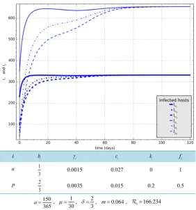
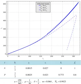
Below, are plots of trajectories of significant components (when the time of the realization of the asymptotic stability is reasonable) of the states of the model (infectious hosts and infectious questing vector) or parametric curves (when the time of the realization of the asymptotic stability is very long) between significant components accompany by finishing sections of trajectories (to show how accurate the result produced by numerical scheme is) representing scenarios corresponding to set of data (with the corresponding values of the 0 computed) given below each figure. The shows in these plots are the asymptotic stability (each scenario is based on three initial states); the effectiveness of the manner various combination of parameters values acts to lower the ende-micity of the malaria in the area. These plots are organized in scenarios based on protecting skills.
5.1.1. Scenarios with One Protected Skill of Two Third of the Hosts with Net with Poor Killing Effect 0.2
k =
Figures 4-11show scenarios where humans are protected with bed nets with small killing effect (i.e. kp =0.2)
i bi γi ci ki fi
n 1
3 0.0015 0.027 0 1
p 2
3 0.002 0.023 0.2 0.8
150 365
a= , 1
30
µ = , 2
3
δ = , m=0.064, 0=339.648
J. C. Kamgang et al.
i bi γi ci ki fi
n 1
3 0.0015 0.027 0 1
p 2
3 0.002 0.023 0.2 0.8
150 365
a= , 1 30
µ= , 2 3
[image:13.595.175.454.81.376.2]δ= , m=0.064, 0=339.648
Figure 5.Infectious vectors components in the scenario inFigure 4.
i bi γi ci ki fi
n 1
3 0.0015 0.027 0 1
p 2
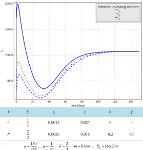
3 0.0035 0.015 0.2 0.5
150 365
a= , 1
30
µ = , 2
3
δ = , m=0.064, 0=166.234
[image:13.595.172.455.402.705.2]i bi γi ci ki fi
n 1
3 0.0015 0.027 0 1
p 2
3 0.0035 0.015 0.2 0.5
150 365
a= , 1
30
µ = , 2
3
[image:14.595.174.454.82.377.2]δ = , m=0.064, 0=166.234
Figure 7.Infectious vectors components in the scenario inFigure 6.
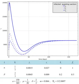
i bi γi ci ki fi
n 1
3 0.0015 0.027 0 1
p 2
3 0.0045 0.009 0.2 0.3
150 365
a= , 1
30
µ = , 2
3
δ = , m=0.064, 0=112.0697
J. C. Kamgang et al.
i bi γi ci ki fi
n 1
3 0.0015 0.027 0 1
p 2
3 0.0045 0.009 0.2 0.3
150 365
a= , 1
30
µ = , 2
3
δ = , m=0.064, 0=112.0697
Figure 9. Infectious vectors components in the scenario in Figure 8.
i bi γi ci ki fi
n 1
3 0.0015 0.027 0 1
p 2
3 0.0065 0.007 0.2 0.05
150 365
a= , 1
30
µ = , 2
3
[image:15.595.175.455.83.380.2]δ = , m=0.064, 0=59.3678
i bi γi ci ki fi
n 1
3 0.0015 0.027 0 1
p 2
3 0.0065 0.007 0.2 0.05
150 365
a= , 1
30
µ = , 2
3
δ = , m=0.064, 0=59.3678
Figure 11. Infectious vectors components in the scenario inFigure 10.
and a repelling effect that increases from poor (see Figure 4, Figure5, where fp =0.8) to a quite high (see
Figure 10, Figure11, where fp =0.05).
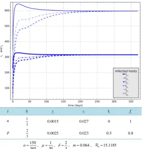
5.1.2. Scenarios with One Protected Skill of Two Third of the Hosts Using Net with Killing Effect
0.5
k =
Figures 12-19show scenarios where the killing effect of bed nets in protection skills is better (kp =0.5) than those in scenario in Figures 4-11.
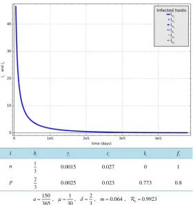
Figures 20-27 are scenarios with one protection skill not corresponding to the section, and which, with parameters values have been chosen in order to compute situation of 0 closed to one. Figures 20-23 are parametric curves (Figure 20, Figure21when 0>1 and Figure 22, Figure23when 0≤1 closed to one) of the dependence between infectious hosts and infectious vectors components of the state of the model, with the finishing section of the corresponding components (Figure 24, Figure25when 0>1 and Figure 26, Figure
27 when 0≤1 closed to one). What is fascinating in these figures is the accuracy of the results produced by the numerical scheme used.
5.1.3. Scenarios with One Protected Skill of Six Seventh of the Hosts Using Net
J. C. Kamgang et al.
i bi γi ci ki fi
n 1
3 0.0015 0.027 0 1
p 2
3 0.0025 0.023 0.5 0.8
150 365
a= , 1
30
µ = , 2
3
[image:17.595.175.455.82.375.2]δ = , m=0.064, 0=15.1185
Figure 12.Scenario with middle killing effect and poor protecting effect.
i bi γi ci ki fi
n 1
3 0.0015 0.027 0 1
p 2
3 0.0025 0.023 0.5 0.8
150 365
a= , 1
30
µ = , 2
3
δ = , m=0.064, 0=15.1185
i bi γi ci ki fi
n 1
3 0.0015 0.027 0 1
p 2
3 0.0035 0.015 0.5 0.5
150 365
a= , 1
30
µ = , 2
3
δ = , m=0.064, 0=7.663
Figure 14. Scenario with better protecting effect than in the previous.
i bi γi ci ki fi
n 1
3 0.0015 0.027 0 1
p 2
3 0.0035 0.015 0.5 0.5
150 365
a= , 1
30
µ = , 2
3
δ = , m=0.064, 0=7.663
J. C. Kamgang et al.
i bi γi ci ki fi
n 1
3 0.0015 0.027 0 1
p 2
3 0.0045 0.009 0.5 0.3
150 365
a= , 1
30
µ = , 2
3
δ = , m=0.064, 0=4.884
Figure 16.Scenario with better protecting effect than in the previous.
i bi γi ci ki fi
n 1
3 0.0015 0.027 0 1
p 2
3 0.0045 0.009 0.5 0.3
150 365
a= , 1
30
µ = , 2
3
δ = , m=0.064, 0=4.884
i bi γi ci ki fi
n 1
3 0.0015 0.027 0 1
p 2
3 0.0065 0.007 0.5 0.03
150 365
a= , 1
30
µ = , 2
3
δ = , m=0.064, 0=2.355
Figure 18.Scenario with better protecting effect than in the previous.
i bi γi ci ki fi
n 1
3 0.0015 0.027 0 1
p 2
3 0.0065 0.007 0.5 0.03
150 365
a= , 1
30
µ = , 2
3
δ = , m=0.064, 0=2.355
J. C. Kamgang et al.
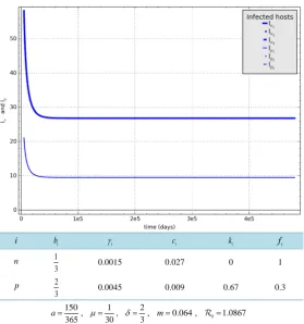
i bi γi ci ki fi
n 1
3 0.0015 0.027 0 1
p 2
3 0.0045 0.009 0.67 0.3
150 365
a= , 1
30
µ = , 2
3
δ = , m=0.064, 0=1.0867
Figure 20.Scenario with better protecting effect than in the previous.
i bi γi ci ki fi
n 1
3 0.0015 0.027 0 1
p 2
3 0.0045 0.009 0.67 0.3
150 365
a= , 1
30
µ = , 2
3
δ = , m=0.064, 0=1.0867
i bi γi ci ki fi
n 1
3 0.0015 0.027 0 1
p 2
3 0.0025 0.023 0.773 0.8
150 365
a= , 1
30
µ = , 2
3
[image:22.595.173.455.82.377.2]δ = , m=0.064, 0=0.9923
Figure 22.Scenario with high killing effect and power protecting effect.
i bi γi ci ki fi
n 1
3 0.0015 0.027 0 1
p 2
3 0.0025 0.023 0.773 0.8
150 365
a= , 1
30
µ = , 2
3
δ = , m=0.064, 0=0.9923
[image:22.595.174.453.407.706.2]J. C. Kamgang et al.
i bi γi ci ki fi
n 1
3 0.0015 0.027 0 1
p 2
3 0.0045 0.009 0.67 0.3
150 365
a= , 1
30
µ = , 2
3
[image:23.595.175.455.80.379.2]δ = , m=0.064, 0=1.0867
Figure 24.Finishing section of trajectories corresponding to Figure 20.
i bi γi ci ki fi
n 1
3 0.0015 0.027 0 1
p 2
3 0.0045 0.009 0.67 0.3
150 365
a= , 1
30
µ = , 2
3
δ = , m=0.064, 0=1.0867
[image:23.595.171.455.405.706.2]i bi γi ci ki fi
n 1
3 0.0015 0.027 0 1
p 2
3 0.0025 0.023 0.773 0.8
150 365
a= , 1
30
µ = , 2
3
[image:24.595.174.455.83.381.2]δ = , m=0.064, 0=0.9923
Figure 26.Finishing section of trajectories corresponding toFigure 22.
i bi γi ci ki fi
n 1
3 0.0015 0.027 0 1
p 2
3 0.0025 0.023 0.773 0.8
150 365
a= , 1
30
µ = , 2
3
δ = , m=0.064, 0=0.9923
[image:24.595.173.455.398.706.2]J. C. Kamgang et al.
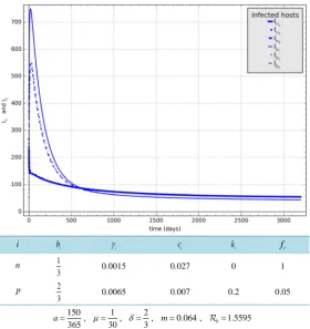
i bi γi ci ki fi
n 1
3 0.0015 0.027 0 1
p 2
3 0.0065 0.007 0.2 0.05
150 365
a= , 1
30
µ = , 2
3
[image:25.595.174.455.82.380.2]δ = , m=0.064, 0=1.5595
Figure 28.Scenario with parameters values of Figure 10.
i bi γi ci ki fi
n 1
3 0.0015 0.027 0 1
p 2
3 0.0065 0.007 0.2 0.05
150 365
a= , 1
30
µ = , 2
3
δ = , m=0.064, 0=1.5595
[image:25.595.173.456.406.707.2]i bi γi ci ki fi
n 1
3 0.0015 0.027 0 1
p 2
3 0.0065 0.007 0.5 0.03
150 365
a= , 1
30
µ = , 2
3
[image:26.595.174.455.82.378.2]δ = , m=0.064, 0=0.0130
Figure 30. Scenario with parameters values of Figure 18.
i bi γi ci ki fi
n 1
3 0.0015 0.027 0 1
p 2
3 0.0065 0.007 0.5 0.03
150 365
a= , 1
30
µ = , 2
3
[image:26.595.171.456.402.706.2]δ = , m=0.064, 0=0.0130
J. C. Kamgang et al.
5.1.4. Scenarios with Two Protected Skills; Half Protected
( )
h and Full Protected( )
pFor scenarios with two protections (h for half protected, and p for full protected), since the components of infectious vectors behave nearly the same as what appears in scenarios with one protection in Figures 4-31
above, we present only figures of trajectories of the infectious hosts components of the state of the system (Figure 32, Figure 33). For chosen values of parameters such that 0 is closed to unity, parametric curves representing infectious hosts variations for three initial states (Figure 34, 0 >1), (Figure 35, 0≤1); since for each, the time of the realization of the asymptotic stability is quite long, the respective finishing sections of each case is also presented for the obviousness of the point each tends to, since the two figures look the same (Figure 36, 0 >1), (Figure 37, 0 ≤1). In Figure 38 is trajectories of infected hosts with parameters of scenarios inFigures 33 with modification in the proportion of protected hosts as a show of how the proportion of bed net users impact on the level of endemicity.
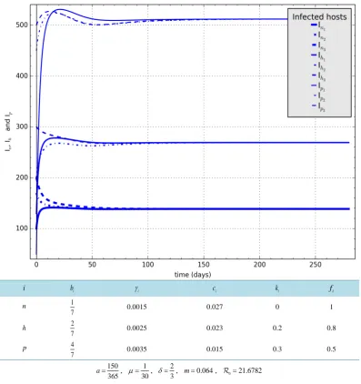
5.1.5. Scenarios with Three Protected Capabilities; Poor Protected
( )
h , Middle Protected( )
mand Full Protected
( )
pFor scenarios with three protections (h for poor protected, m for middle protected and p for full protected),
i bi γi ci ki fi
n 1
7 0.0015 0.027 0 1
h 2
7 0.0025 0.023 0.2 0.8
p 4
7 0.0035 0.015 0.3 0.5
150 365
a= , 1
30
µ = , 2
3
δ = , m=0.064, 0=21.6782
Figure 32. Scenario with lower killing effect and poor protecting effect for h—protection strategy and
[image:27.595.115.513.273.696.2]