Global Convergence of a Modified Tri Dimensional Filter Method

http://dx.doi.org/10.4236/am.2015.62023

Global Convergence of a Modified

Tri-Dimensional Filter Method

Bei Gao, Ke Su, Zixing Rong

Department of Mathematics and Information Science, Hebei University, Baoding, China Email: [email protected], [email protected], [email protected]

Received 9 January 2015; accepted 27 January 2015; published 3 February 2015

Copyright © 2015 by authors and Scientific Research Publishing Inc.

This work is licensed under the Creative Commons Attribution International License (CC BY).

http://creativecommons.org/licenses/by/4.0/

Abstract

In this paper, a tri-dimensional filter method for nonlinear programming was proposed. We add a parameter into the traditional filter for relaxing the criterion of iterates. The global convergent properties of the proposed algorithm are proved under some appropriate conditions.

Keywords

Tri-Dimensional, NCP Function, Global Convergence, QP-Free

1. Introduction

This paper is concerned with finding a solution of a Nonlinear Programming (NLP) problem, as following

( )

( )

min

. . 0, f x

s t c x ≤ (1) where f x

( )

:Rn→R ,

( )

(

1

( )

, ,

( )

)

T:

n m

m

c x = c x  c x R →R are second-order continuously differentiable. The Lagrangian function associated with problem (1) is the function

( )

,

( )

( )

L xλ = f x +λc x

where

(

1, 2, ,

)

T m

m R

λ= λ λ  λ ∈ is the multiplier vector. For simplicity, we denote the column vector

(

_xT_,λT

)

T as

( )

x,λ . A point

(

_x∗,λ∗

)

∈_Rn m×

is called a Karush-Kuhn-Tucker (KKT) point if it satisfies the following conditions:

(

,

)

0,

( )

0, 0,

( )

0,

xL x λ c x λ λ c x

∗ ∗ ∗ ∗ ∗ ∗

∇ = ≤ ≥ = (2)

we also say that x∗∈D is a KKT point of problem (1) if there exists a λ∗_∈Rm

(2).

Traditionally, this question has been answered by using penalty function. But it is difficult to find a suitable penalty parameter. In order to avoid the pitfalls of penalty function, Nonlinear programming problems (NLP) filter methods were first proposed by Fletcher in a plenary talk at the SIAM Optimization Conference in Victoria in May 1996; the methods are described in [1]. And soon, Global convergence proof of filter method was given in [2]. Because of good global convergence and numerical results, filter methods have quickly become popular in other areas such as nonsmooth optimization, nonlinear equations and so on [3] [4].

Motivated by the ideas of filter methods above, a tri-dimensional filter method for nonliner programming was proposed as acceptance criterion to judge whether to accept a trial step in our algorithm. We have following ad-vantages:

1) By enhancing the flexibility of filter, motivated by [5], we increase a dimension by introducing a parameter to relax the criterion of iterates.

2) The Maratos effect that makes good progress toward the solution may be rejected and has been avoided by using tri-dimensional filter method as acceptance criterion.

3) Tri-dimensional filter method can make full use of the information we get along the algorithm process. This paper is divided into 4 sections. The next section introduces the concept of a Modified tri-dimensional filter and the NCP function. In Section 3, an algorithm of line search filter is given. The global convergence properties are proved in the last section.

2. Preliminaries

2.1. NCP Function

The method that based on the Fischer-Burmeister NCP function are efficient, both theoretical results and com-putational experience. The Fischer-Burmeister function has a very simple structure

( )

2 2

, .

a b a b a b

ψ = + − −

We know that: ψ is continuously differentiable everywhere except at the origin, but it is strongly semis-mooth at the origin. i.e. if a≠0 or b≠0, then ψ is continuously differentiable at

( )

a b, ∈R2, and

( )

2 2 2 2

, a 1, b 1 ;

a b

a b a b

ψ  

∇ =_ − − _

+ +

 

if a=0 and b=0, then the generalized Jacobian of ψ at

( )

0, 0 is

( )

{

2 2

}

0, 0 1, 1 1 .

ψ ξ η ξ η

∂ = − − + =

Let

(

,

)

(

( )

,

)

, 1

i x c xi i i m

φ µ =ψ − µ ≤ ≤

We denote

(

)

(

(

(

)

)

(

(

)

)

)

T

T T

1

, _x , , ,

x µ L x µ xµ

Φ = ∇ Φ , where Φ1

(

x,µ

)

=

(

φ1

(

x,µ

)

,,φm

(

x,µ

)

)

T.

Clearly, the KKT optimality conditions (2) can be equivalently reformulated as the nonsmooth equations

(

x,µ

)

0

Φ = .

If

(

c x_i

( )

,µ_i

)

≠

( )

0, 0 , then φl is continuously differentiable at

(

,

)

n m

x µ ∈R + . In this case, we have

( )

( )

(

)

2 ₂ 1

( )

;

(

( )

)

2 ₂ 1

i i

x i i i i

i i i i

c x

c x e

c x c x

µ

µ

φ φ

µ µ

   

−

   

∇ =_ + ∇_ ∇ =_ − _

 +   + 

   

where e_i =

(

0,, 0,1, 0, 0

)

T∈Rm is the ith column of the unit matrix, its ith element is 1, and other elements are 0.

If c xi

( )

=0 andµi =0,1≤ ≤i m, then φi

(

x,µ

)

is strongly semismooth and directionally differentiable at

(

,

) (

{

1

)

( )

1 1

}

x iφ x µ ξ c xi ξ

∂ = + ∇ − ≤ ≤

and

(

,

) (

{

1

)

1 1 .

}

i i x

µφ µ ξ ξ

∂ = − − ≤ ≤

We may reformulated the KKT (at point x*,λ µ*, *) conditions as a system of equations.

(

* * *

)

(

* *

)

1

, , 0, , 0,

xL x λ µ x µ

∇ = Φ =

where

(

1, 2, ,

)

T

p

p R

λ= λ λ _ λ ∈ and

(

1 2

)

T

, , , m Rm

µ= µ µ  µ ∈ are the multiplier vectors,

(

,

)

(

( )

,

)

,

i x j g xi j

φ µ =ψ − µ

(

* *

)

(

(

*

) (

*

)

(

*

)

)

1 1 2 2

, , , , , , m , m

x x x x

φ µ = φ µ φ µ φ µ .

Replace the violation constrained function p G x

(

( )

)

in filter F of Fletcher and Leyffer method, we use the violation constrained function p G x

(

( )

,µ

)

= Φ1

(

x,µ

)

2.

If

(

( )

k , k

)

( )

0, 0 c x µ ≠ , let

(

)

( ) ( )

2 2

(

)

( ) ( )

2 2

, 1; , 1;

k k

j j

k k k k k k

j j j j

k k k k

j j j j

c

x x

c c

µ

ξ ξ µ η η µ

µ µ

−

= = + = = −

+ +

otherwise we denote

(

)

2

(

)

2

, 1 ; , 1 .

2 2

k k k k k k

j j x j j x

ξ =ξ µ = + η =η µ = − +

Let

( )( )

( )

11 12

T 21 22

.

diag diag

k k

k k

k k k k k k

H c

V V

V

V V ξ c η

 ∇ 

 _{  }

= _{ }= _

∇

 _{  }

where Hk is a positive matrix which may be modified by BFGS update. diag

( )

ξk

or diag

( )

ηk

denotes the diagonal matrix whose j diagonal element is ξk or ηk respectively.

Definition 1.1 [1] A pair

(

f h_j, _j

)

is said to dominate another pair

(

f hl, l

)

if and only if both fj≤ fl and

j l

h ≤h .

Definition 1.2 [1] A filter is a list of pairs

(

f hl, l

)

such that no pair dominates any other. A point

(

f hj, j

)

is said to be acceptable for inclusion in the filter if it is not dominated by any point in the filter.

Definition 1.3 NCP pair and NCP functions [6]We call a pair

( )

2 ,

a b ∈R to be an NCP pair if a≥0, 0

b≥ and ab=0 a function ψ :R2→R is called an NCP function if

( )

a b, =0 if and only if

( )

a b, is an NCP pair.

Denote h x

( )

= Φ1

(

x,µ

)

2 in the following context. It is straightforward to see that the constraint (1) is equivalent to the following equation: h x

( )

=0.

2.2. Tri-Dimensional Filter

A two dimensional filter is often used in traditional filter method, some information about convergent like the positions of iterates are neglected. Therefore, we aim to enhance its flexibility of filter. Motivated by [5], we adopt

(

h f, ,δ

)

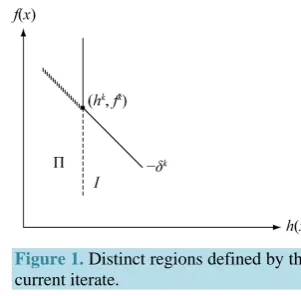
in which a parameter δ is used to relax the criterion of iterates. We denote the filter by k for each iteration k. Flexible exact penalty function is introduced to promote convergence refer to [7]. Given a prescribed interval, penalty parameter can be chosen as any number from it and it is extends classical penalty function methods. We generalized the idea to filter which we called Tri-dimensional filter. Different from the original two dimensional filter, we increase a dimension by introducing a parameter.

We use pairs

(

h_j,f_j,δ_j

)

to constitute the elements of filter, where δj is a non-negative parameter. Our

strategy for setting δj depends on the region in h− −f δ space to which sk moves into.Figure 1 is Dis-tinct regions defined by the current iterate.

If sk moves into region I, which is defined as

(

)

{

, , : 1.1 _k and _{k k k k}, _k 0 ,

}

[image:4.595.232.383.84.232.2]

Figure 1. Distinct regions defined by the current iterate.

We say that the algorithm does not make good improvement since we do not want to accept points with larger constraint violation. Thus, we try to impose stricter acceptance criterion. Meanwhile, we do not permit δk larger than σk. In our algorithm, we increase

k

δ in the following way

(

)

(

)

1 min , max 0.001, 0.1 .

k k k

k k k k

k k k

f f x s

h h x s

δ + σ δ δ

   − + 

  

=  +  _{ − +} − _

   

 

(3)

If sk moved into region Π which is defined as

(

)

{

h f, ,δ :h 0.9h_k and f δ_kh f_k δ_kh_k,δ_k 0 ,

}

Π = < + < + ≥

We say that the algorithm makes good improvement since it reduces not only the constraint violation, but also the penalty function value. So, we may loosen the acceptance criterion to wish more improvement. Here, we achieve this goal by reducing δk by setting

(

)

(

)

1 max 0, max 0.001, 0.1 .

k k k

k k k

k k k

f f x s

h h x s

δ ₊ =  σ −  _ −_{− +}+ −δ _

   

 

4)

In our algorithm, the trial step sk is accepted by filter if

(

_{k k}

)

_j or

(

_{k k}

)

_j

(

_{k k}

)

(

_{j j}

)

and _k 0

h x +s ≤γh f x +s +δ h x +s ≤γ f +δ δ ≥ (5) For all

(

h_j,f_j,δ_j

)

∈_k. The parameter γ ∈

( )

0,1 is a constant close to 1 which sets an “envelope” around the border of the dominated part of the

(

h f, ,δ

)

-space in which the trial step is rejected. And also in the filter if

and and 0

j k j k j k k k k

h >h h +δ f >h +δ f δ ≥ (6) then we say xj is dominated by xk.

3. Description of the Algorithm

In this section we hope that the Lagrange multiplier λk will converge to the Lagrange multiplier λ ∗

at the solution x∗. From the KKT system of (1), a good estimate of the Lagrange multiplier is the least square solu-tion of c x

( )

−A x

( )

λ=0, namely λ=

(

A x

( )

)

+c x

( )

. In our algorithm, λk is updated only after a trial step is accepted, and is set componentwise as

(

)

{

}

(

)

{

}

, ,

max , 0 , 0, ,

min , 0 , , 0,

i i i

k k i

i i i

k k k

i

i i

k k

A c l u

A c l u

A c l u

λ +

+

+ 

 =



=_ = = +∞



 _{= −∞ =}



(7)

satisfied, and the second order sufficient conditions are satisfied. Then when

1, σ _> λ∗

x∗ is the strict local minimizer of penalty function. So we force the condition at each iteration: σk+1≥ λk+1 1.

And also, since the penalty term aims to reduce the constraint violation we double the penalty parameter if the constraint violation could not reduce by half, that is

(

)

1 2 , if 0.5 .

k k h xk sk hk

σ ₊ = σ + ≥

To summarize, we update the penalty parameter in the following formula:

{

}

(

)

{

1 1

}

1

1 1

max 2 , , 0.5 ,

max , , otherwise.

k k k k k

k

k k

h x s h

σ λ σ σ λ + + +  _{+ ≥}  = 

 (8)

The improved algorithm is presented as following.

Algorithm

Step 0. Initialization: Give a starting point 0

n

x ∈R , µ0, λ0 and a initial positive definite matrix H0,

( )

0,1

τ ∈ , k=0. compute h0,f g0, 0,A0.

Step 1. Terimination test. If hk+ gk−Akλk _∞ <ε then returing xk as a solution and stop.

Step 2. Computation of the search direction. compute _dk0 _and λk0 _{by solving the following linear system}

in

(

d,λ

)

:

. 0 k k d f V λ −∇    =    

    (9) where ∇_fk = ∇_{f x}

( )

k

.

If _dk0 =_{0, then stop otherwise, compute}

(

_dk1_,λk1

)

_{by solving the following linear system in}

(

_d,λ

)

_:

1 . k k k d L V λ −∇    =  

  _−Φ

    (10)

where ∇ = ∇Lk L x

(

k,λk

)

and 1 1

(

,

)

k k k

x λ

Φ = Φ .

Step3. Liner search with filter If 1 0

k

Φ = then let bk =1 and ρ =k 0, otherwise if _dk0 =_{0 then let b}k =_{0 and} ρ =k _{1, otherwise de-}

note bk = −

(

1 ρk

)

and

( )

( )

(

)

( )

(

)

0 1 0 0 1 T T T T 1 if 1 otherwise k

k k k

k _{k k}

k k k

d f d f

d f

d d f

θ ρ θ  _{∇ ≤ ∇}   =  ∇ −   − ∇  (11) and let 0 1

0 1 ,

k k

k

k k

k k

k

d d d

b ρ

λ λ λ

   

 

= _{ }+ _{ }

 

     

Step 4. Acceptance criterion of the trial step Let x xk sk

+ _{= +}

, evalute h+ and f+ andδ+; If x+ is accepted by filter, xk 1 x +

+ = and go to step 5;

1

k k

x₊ =x , and k= +k 1; go to step 2.

Step 5. Paramenters update

Update λk+1 by (7); Update σk+1 by (8); Update δk+1 by (3) or (4); k= +k 1 go to step 1.

4. The Convergence Properties

To present a proof of global convergence of algorithm, in this section, we always assume that the following conditions hold.

A2 f andg_i are twice Lipschitz continuously differentiable, and for all y z, ∈Rn m+ ,

( )

( )

3 ,

( )

( )

3 ,

L y L z m y z y z m y z

∇ − ∇ ≤ − Φ − Φ ≤ −

where m3 >0 is the Lipschitz constant.

A3 Hk is positive definite and there exist positive numbers m1 and m2 such that

2 T 2

1 2

k

m d ≤d H d≤m d

for all _d∈_Rn

and all k.

Lemma 1. If Φ ≠k 0

then _Vk

and _V*

are nonsingular.

Proof. If k 0, u V

ϑ  ₌  

  for some

(

,

)

n

uϑ ∈R , where ϑ=

(

ϑ1,,ϑ

)

T,u=

(

u1,,un

)

T, then we have

0

k k

H u+ ∇c v= (12) and

( )( )

T

( )

diag ξk ∇ck u+diag ηk v=0 (13) From the definition of ξkj and

k j

η , we know that ξ ≥kj 0 and 0

k j

η ≠ for all j. So, diag ηk is nonsingu-lar. We have

( )

(

)

1

( )( )

T

diag k diag k k

v= − η − ξ ∇c u (14)

Putting (14) into (12), we have

(

)

( )

(

( )

)

1

( )

T

T T T

diag diag 0

k k k k k k k

u H u+ ∇c v =u H u u− ∇c ξ η − ∇c u=

The fact that −∇ckdiag

( )

ξk

(

diag

( )

ηk

)

−1

( )

∇ck T is positive semidefinite implies u=0, and then v=0 by (14). Vk is nonsingular. And if

(

x*,µ*

)

is an accumulation point of

{

(

k, k

)

}

x µ ,

{

(

k, k

)

}

(

*, *

)

x µ → x µ ,

* k

Φ → Φ and VK →V*. If Φ ≠* 0 then Φ* is nonsingular. This lemma holds.  The lemma 2 hold (see [8] Lemma 2)

Lemma 2. If _dk0 =_{0, then} ∇_{f x}

( )

k =_{0. and x}k _{is KKT point of problem (NLP).} Lemma 3. Consider an infinite sequence iterations on which

{

1 2,

}

k k

f

Φ entered into filter, where 2

1 0

k

Φ > and

{ }

fk is bounded below. It follows that 1 0

k

Φ → .

Proof. Suppose the theorem is not true, then exists an ε >0 and an infinitely members of index set K such that either 1

(

,

)

0

k k

x µ ε

Φ ≥ > and 1

(

1, 1

)

1

(

,

)

k k k k

x+ µ + η x µ

Φ ≤ Φ for any k∈K . then we obtain that

(

)

{

1 ,

}

0

k k

k K x µ

∈

Φ → , or

{ }

fk k K∈ is monotonically decreasing, then lemma 5.1 implies 1

(

,

)

0

k k

x µ

Φ → .

So, the lemma holds. 

The following lemma 4 - 5 hold (see [9])

Lemma 4. dk →0.

Lemma 5. If

(

x*,µ*

)

is an accumulation point of

{

(

xk,µk

)

}

then d*=0, and d*,λ* is the solution of: *

* .

0

d f

V λ

−∇   

=  

 

   

and _{∇L x}

(

*_,µ*

)

₌₀ .

Theorem 1. If

(

_x*_,µ*

)

is an accumulation point of

{

(

k, k

)

}

x µ then _x*

is a KKT point of Problem (NLP). It is obviously to prove the conclusion holds according to the above lemmas.

Acknowledgements

Foundation of China (No. 11101115), the Natural Science Foundation of Hebei Province (No. 2014201033) and the Science and Technology project of Hebei province (No. 13214715).

References

[1] Fletcher, R. and Leyyfer, S. (2002) Nonlinear Programming without a Penalty Function. Mathematical Programming, 91, 239-269. http://dx.doi.org/10.1007/s101070100244

[2] Fletcher, R., Leyffer, S. and Toint, P.L. (1998) On the Global Convergence of an SLP-Filter Algorithm. Numerical Analysis Report NA/183, University of Dundee, Dundee.

[3] Fletcher, R., Leyffer, S., et al. (2006) A Brief History of Filter Methods.Mathematics and Computer Science Division, Preprint ANL/MCSP1372-0906, Argonne National Laboratory.

[4] Chin, C.M., Rashid, A.H.A. and Nor, K.M. (2007) Global and Local Convergence of a Filter Line Search Method for Nonlinear Programming. Optimization Method Software, 22, 365-390. http://dx.doi.org/10.1080/10556780600565489 [5] Wang, X. (2010) A New Filter Trust Region Method for Nonlinear Programming. Journal of the Operations Research

of China, 10, 133-140.

[6] Zhou, Y. and Pu, D. (2007) A New QP-Free Feasible Method for Inequality Constrained Optimization. OR Transac-tions, 11, 31-43.

[7] Curtis, F.E. and Nocedal, J.(2008) Flexible Penalty Function for Nonlinear Constrained Optimization. IMA Journal of Numerical Analysis, 28, 749-769. http://dx.doi.org/10.1093/imanum/drn003

[8] Su, K. (2008) A New Globally and Superlinearly Convergent QP-Free Method for Inequality Constrained Optimization. Journal of Tongji University, 36, 265-272.