Automated Tuning and Controller Design for DC DC Boost Converter

(1)

Automated Tuning and Controller Design for DC-DC Boost Converter

B. Amarendra Reddy

1

_{, M.S.V. Santosh Kumar}

2

1,2

_{Dept. of Electrical & Electronics Engineering, Andhra University, AP, India}

---*---Abstract -**

Design of Controller of any converter plays an important role in effective disturbance rejection, noise attenuation etc. MATLAB based SISOTOOL provided an effective way of designing controller and also provides optimizing the parameters of the controller. In this paper the procedural steps are given to design a controller and to tune the control parameters.

Key Words: Controller Design, Tuning Methods, MATLAB Simulation, Steep Descent, Loop Shaping, IMC Tuning.

1. INTRODUCTION

In SMPS (Switched-mode power supply) DC-DC boost converter has played very important to handle high power. Boost converters are used in many applications for regulated power supply. In some applications output changes due to isolation level, temperature change etc, and in other applications output changes according to discharging characteristics and the load change. So there is need for controller for boost converter in many applications.

The controller is designed using MATLAB sisotool(single input single output). Sisotool opens the SISO Design Tool with root locus view and Bode diagram. The controller parameters are optimized by tuning. Manual tuning is purely trail and error process, time consuming and non - systematic. It may not produce optimal design and can lead to dangerous conditions. Sisotool has some standard design procedures for tuning the parameters of the controller.

This paper is organized as follows: - The controller design and tuning methods are described in section 2 and 3. Examples shown are described in section 4. Conclusion is given in section 5.

2. DESIGN OF CONTROLLER

The design process using SISO Tool in MATLAB environment includes the following points

Step 1:The compensator elements are to be optimized for example Gain, Real Pole, Real Zero, Complex Zeros, Complex Poles etc.

Step2:Choose the type of the design requirement for example Step response bounds/Step response lower/ upper amplitude limit, Impulse Response lower/ upper amplitude limit, Bode magnitude upper/lower Limit, Phase Margin.

Step3:The response specifications for the design requirement are to be specified for example the PM and GM

in Frequency Response Specifications (OR) Specify rise time, settling time, Peak Overshoot in Time Response Specifications

Step4:Type of response is to be specified for example closed loop from r to y/closed loop from r to u/compensator C/ Input sensitivity/Noise sensitivity/open loop/output sensitivity).

Step5: We have choose the method for optimization like Gradient search method (or Pattern Search method or Simplex Search method) and Maximum number of iterations and function tolerance etc.

Step6:As a final step the optimization can be started by clicking button. After successful termination with desired convergence, we obtain the compensated transfer function.

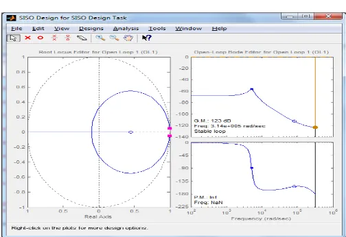
[image:1.595.305.560.379.737.2]

Fig -1: Command of sisotool in workspace

[image:1.595.307.559.547.720.2]

(2)

(b)Corresponding Bode plot

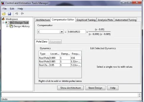
Fig -4: Transfer function in compensator editor.

3. AUTOMATED TUNING

For automated tuning leading edge boost converter system transfer function and the open–loop frequency response specifications are to be noted. Optimization Based Tuning is to create an initial compensator design (or) to refine the current compensator design. In the Optimization Based Tuning there are three important steps

(i) Selecting the compensators to optimize. (ii) Select the design requirements.

(iii) Select the Optimizing options and Optimize.

3.1 Steepest Descent Method

The classical steepest Descent method is one of the oldest methods for minimization of a general nonlinear function .The steepest descent method is also known as gradient descent method was first proposed by Cauchy in 1847.The basis for the method is the continuous function should decrease at least initially if one takes a step along the direction of the negative gradient.

3.2 Simplex Search Method

Simplex-based direct search methods are based on comparison of the objective function values at the vertices of a simplex (which is a set of n+ 1 point in dimension n) that is updated by the algorithms steps.

3.3 IMC Tuning Method

It obtains a full-order stabilizing feedback controller using the IMC design method. A Control System design is expected to provide a fast and accurate set point tracking that is output of the system should follow the input as closely as possible. Also any external disturbances must be corrected by control system as efficiently as possible. In practice an open loop system is sensitive to modeling errors and inability to deal with external disturbances entering the system. To deal with disturbances and modeling error, control systems are always of closed loop type. A design strategy is to shape directly the relevant closed loop transfer functions. Specify the desired closed loop response and solve for resulting controller. The key step is to specify a good closed- loop response.

3.4 Loop Shaping Method

It finds a full-order stabilizing feedback controller with a desired open loop bandwidth or shape.

Principle of Loop Shaping: This is the classical approach in which the magnitude of the open loop transfer function is shaped. Usually no optimization is involved and the designer aims to obtain magnitude of loop gain with desired band width, slopes. Loop Shape refers to the magnitude of the loop transfer function as a function of frequency. By loop shaping we mean a design procedure that involves explicitly shaping the magnitude of the loop transfer function.

4. EXAMPLES

To show the effectiveness of these stabilizing PI controller design methods third-order systems are considered for simulation in MATLAB.

4.1 Steepest Descent Method

Original Compensator Transfer Function: (Which is to be refined)

6.535(z -1.985z+0.987)

2

(z-1)(z-0.8008)

After fine adjustments by changing the pole zero locations in the vicinity of original compensator after compensation

2

3.4605(z -1.969z+0.9718)

(z-1)(z-0.7071)

[image:2.595.41.284.317.489.2]

(3)

Input Perturbation: Initially the system Operates with an input of 10V DC Supply and it is perturbed with a step change of 10volts to 15 volts at 50 milliseconds.

Chart -1: Input Disturbances of SD method

Observations:

The system with original compensator is exhibiting more overshoot and it takes more settling time after input perturbation at 50 milliseconds.

The system with Steepest Descent method optimized compensator is exhibiting lesser overshoot and less settling time after input perturbation at 50 milliseconds.

Case (b) : Load Disturbances:

Initially the system Operates with a load resistance of 10 ohms and it is perturbed with a step change of 10 ohms to 110 ohms at 50 milliseconds.

Chart -2: Load Disturbances of SD method

Observations:

The system with original compensator is exhibiting more overshoot after load disturbance at 50 milliseconds.

The system with Steepest Descent method optimized compensator exhibiting overshoot less than the system with original

4.2 Simplex Search Method

2

6.535(z -1.985z+0.987)

(z-1)(z-0.8008)

2

4.038(z -1.986z+0.989)

(z-1)(z-0.7723)

With this compensator the Open loop system is having GM 6.74dB PM 36.6 degrees

Case (a) : Input Disturbances:

Chart -3: Input Disturbances of SS method

Observations:

The system with Simplex Search method optimized compensator is exhibiting lesser overshoot and less settling time after input perturbation at 50 milliseconds.

(4)

Observations:

The system with Simplex Search method optimized compensator exhibiting overshoot less than the system with original

4.3 IMC Tuning Method

Chart -5: Input Disturbances of IMC method

Observations:

The system with IMC tuning method optimized compensator is exhibiting lesser overshoot and less settling time after input perturbation at 50 milliseconds.

Chart -6: Load Disturbances of IMC method

Observations:

The system with original compensator is exhibiting more overshoot after load disturbance at 50 milliseconds. The system with IMC method optimized compensator exhibiting overshoot less than the system with original

4.4 Loop Shaping Method

2

(z-1)(z-0.3333)

7.704(z -1.985z+0.9872)

2

(z-1)(z-0.8008)

6.535(z -1.985z+0.987)

2

(z-1)(z-0.5445)

0.94667(z+1)(z -1.985z+0.9872)

2

(z-1)(z-0.8008)

(5)

input of 10V DC Supply and it is perturbed with a step change of 10volts to 15 volts at 50 milliseconds.

Chart -7: Input Disturbances of LS method

Observations:

The system with loop shaping method optimized compensator is exhibiting lesser overshoot and less settling time after input perturbation at 50 milliseconds.

Chart -8: Load Disturbances of LS method

Observations:

The system with IMC method optimized compensator exhibiting overshoot less than the system with original

5. CONCLUSIONS

Controller is designed using SISO tool. The parameters of controller resulted from this tool is modified using Automated tuning. This automated tuning allows parameter's optimization, parameter's tuning for robust time response and shaping the frequency response for desired bandwidth etc. Here the controller parameters are optimized.

The performance of a DC-DC converter is evaluated using original compensator and different possible compensators against input disturbances and load disturbances.

REFERENCES

[1] Jaen, Carles, et al. "A linear-quadratic regulator with integral action applied to pwm dc-dc converters." IEEE Industrial Electronics, IECON 2006-32nd Annual Conference on. IEEE, 2006

[2] Dragan Maksimovic, Senior Member, IEEE, and Regan Zane, Senior Member, IEEE“ Small-Signal Discrete-Time Modeling of Digitally Controlled PWM Converters”IEEE TRANSACTIONS ON POWER ELECTRONICS, VOL. 22, NO. 6, NOVEMBER 2007.

[3] V. Yousefzadeh, M. Shirazi, and D. Maksimovic, “Minimum phase response in digitally 870. controlled boost and flyback converters,” in Proc. IEEE Appl. Power Electron. Conf., 2007.

[4] Maksimovic, Dragan, and Regan Zane. "Small-signal discrete-time modeling of digitally controlled DC-DC converters." Computers in Power Electronics, 2006. COMPEL'06. IEEE Workshops on. IEEE, 2006.

Automated Tuning and Controller Design for DC DC Boost Converter