Optimization of Precast Post tensioned Concrete I Girder Bridge

(1)

Optimization of Precast Post-tensioned Concrete I-Girder Bridge

Prakash D. Mantur

1

_{, Dr. S. S. Bhavikatti}

2

1

_{PG Scholar, Department of Civil and Environmental Engineering, K.L.E Technological University Hubballi,}

Karnataka, India

2

_{Professor, Department of Civil and Environmental Engineering, K.L.E Technological University Hubballi,}

Karnataka, India

---*---Abstract -**

Bridge is a structure providing passage over an

obstacle without closing the way beneath. Bridges are mainly categorized based how the forces are distributed through the structure, purpose and material availability etc.PSC bridges are adopted for spans between 20m to 40m. The various parameters like selection of design vehicle, position of vehicle and load combination is decided as per IRC:6-2014, deck slab is designed with reference to IRC:21-2000 and the girder is designed with reference to IRC:18-2000, IS:6006-1983, IS:12468 & IS:1343-2012. Parabolic tendon profile is adopted. A computer program is developed in C-programming language to design the deck slab and PSC I-girder. Optimization is carried out by using improved move limit method of sequential linear programming.

Key Words: Post-tensioned, Deck slab, I-Girder, C-Program, Optimization, Improved move limit method.

1. INTRODUCTION

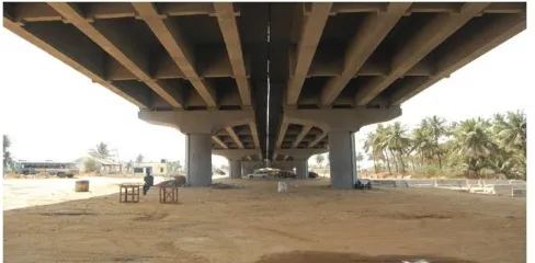
[image:1.595.35.279.548.668.2]

Bridge is a structure providing passage over an obstacle without closing the way beneath. Precast post-tensioned concrete girder bridge is a kind of bridge wherein the I-girders rest on the bearings and deck slab is connected to girder through shear connector.These bridges are generally adopted when the span lies between 20m-40m. PSC bridges give better shear resistance than RCC Bridge because of introducing pre-stressing force to the concrete.

Figure 1.1: Typical I-girder bridge

1.1 IRC vehicles

The live load to be considered for bridge design, particularly for roadways are specified in IRC:6-2014. The various differentiating parameters between different IRC vehicles are, loading, ground contact area and side clearance.

The various IRC vehicles are specified in IRC:6-2014 are,

(a) IRC class AA

 Tracked, with loading of 70 tonnes.

 Wheeled, with loading of 20 tonnes for single axles & 40 tonnes for two axles

(b) IRC class 70R

 Tracked, with loading of 70 tonnes.  Wheeled, with loading of 100 tonnes.

(c) IRC class A train of vehicles with loading of 67.6 tonnes.

(d) IRC class B train of vehicles with loading of 40.5 tonnes.

1.2 Need for optimization

There are many acceptable designs for a single design problem but among all the acceptable designs, one which is most economical will satisfy both structural engineering standards as well as economical need. The act of obtaining the best results under given circumstances is called optimization. Optimization has got huge scope in structural engineering. In this project the cost optimization of precast post tensioned concrete I-girder bridge is carried out.

1.3 Objectives

The various objectives to be achieved are, To employ improved move limit method of sequential linear programming optimization technique for optimum design of precast post-tensioned concrete I-girder.

 To provide the bases for selection of economical dimension in designing of precast post-tensioned concrete I-girder to the structural engineer.  To study the effect of change in grade of concrete

and steel on economy of precast post-tensioned concrete I-girder.

 To carry out the parametric study on effect of cost ratio on optimum design.

2. DESIGN REQUIREMENT

(2)

tensioning the steel reinforcement.

2.1

Check for ultimate moment and shear

Ultimate moment check

Strength of prestressed concrete structure will be checked against the failure conditions. The ultimate moment is calculated as follows,

Ultimate moment with reference to IRC: 18-2000

Ultimate moment under normal condition = 1.25DLBM + 2 SDLBM + 2.5LLBM

Ultimate moment under severe condition = 1.5DLBM + 2 SDLBM + 2.5LLBM

Where,

DLBM=Dead Load Bending Moment

SDLBM=Superimposed Dead Load Bending Moment LLBM=Live Load Bending Moment

in flexure irrespective of the magnitude of cracking moment at the concrete section considered (Mt), and the lesser value taken and, if necessary, shear reinforcement provided. Ultimate shear with reference to IRC:18-2000.

Ultimate shear under normal condition = 1.25 DLSF + 2 SDLSF + 2.5 LLSF

Ultimate shear under severe condition = 1.5 DLSF + 2 SDLSF + 2.5 LLSF

Where,

DLSF = Dead Load Shear Force

SDLSF = Superimposed Dead Load Shear Force LLSF = Live Load Shear Force

3. Design problem

To facilitate development of computer program and checking the program developed the following design is considered.

Preliminary data: Effective span = 30 m Width of road = 7.5 m

Footpath = 1.5 m wide on each side Depth of wearing coat = 80 mm Grade of concrete = M40

Cube strength at transfer = 40 N/mm2

Density of concrete = 24 kN/m3 Density of wearing coat = 22 kN/m3

Parabolic tendon profile is adopted

Cube strength at transfer fci = 0.8fck = 32 MPa. As per IRC:18-2000

Allowable compressive stress in concrete at initial transfer of prestress fct = 0.5fci = 16 MPa

Permissible compressive stress in concrete under service loads fcw = 0.33fck = 13.2 MPa

Allowable tensile stress in concrete at initial transfer of prestress ftt = 0 MPa.

Allowable tensile stress in concrete under service loads ftw= 0 MPa.

Ec = 5000 = 31.622 kN/m2

Duct diameter do = 90 mm Clear cover dc = 50 mm

Allowable stresses in prestressing steel:

Ultimate tensile stress in steel Fp = 1862.14 MPa, Loss ratio = 0.85

[image:2.595.311.558.170.283.2]

Modulus of elasticity in steel E = 2×105_MPa

Figure 3.1: Cross section of deck slab and girder

As carriageway width is 7.5 m and from IRC:6-2014 the live load combination for analysis of deck slab and girder should be critical of 1 lane of 70R or 2 lanes of class A vehicle. The final design forces are,

Table 3.1:Design bending moment

DLBM (kNm)

Class AA

(T)kNm (W)kNm ClassAA ClassA kNm BM (kNm) Design OG 5286.37 2074 1315.44 2361.2 7647.58

IG 5286.37 1596 978.48 1817.2 7103.57

Where,

OG=Outer girder, IG=Inner girder

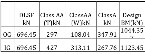
Table 3.2: Design shear force.

DLSF

kN

Class AA

(T)kN

ClassAA

(W)kN

ClassA

kN

BM(kN)

Design

OG 696.45

297 108.04 347.91

1044.35

₇

IG 696.45

427 313.11 267.76 1123.45

3.1

Design program

[image:2.595.310.554.562.654.2]

(3)

3.2 Mathematical formulation of optimization

problem

Mathematical form of general optimization problem involves in finding the variable vector,

to minimize the objective function Z=f(x) subjected to constraints:

gj(x) ≤ 0, where j =1,2 ...m

Where,

x = Design vector with n-dimensions. Z = Objective function.

gj(x) = Inequality constraints of m number.

There are three basic elements required to formulate the optimization problem mathematically they are design variables, objective functions and constraints.

3.3 Design variables

The design variables are,

 Over all depth of girder(X1).  Breadth of top flange(X2).  Depth of top flange(X3).  Breadth of bottom flange(X4).  Depth of bottom flange(X5).

3.4 Objective function

The objective function considered is the minimization of material cost and is assembled as shown below,

Fcost=Qconc * Cconc + Qsteel * Csteel + Qcable * Ccable Where,

Fcost = Optimum cost of girder in lakhs Qconc = Quantity of concrete in m3 Cconc = Cost of concrete in Rs/m3 Qsteel = Quantity of steel in tonnes Csteel = Cost of steel in Rs/tonnes

Qcable = Quantity of cable (prestressing steel) in tonnes Ccable = Cost of cable (prestressing steel) in Rs/tonnes

3.5

Cost consideration

In general the various cost to be considered are from Schedule of Rates(SR) of latest version and the region in which the site belongs to, for example if a site is in Hubballi then we need to refer schedule of rates 2016-2017 public works, ports & inland water transport department, north zone, Dharwad.

The various cost considered are,

For M40 grade of concrete cost is 6,000 Rs/m3, Cost of steel (Fe415 TMT) is 45,000 per Tonne, Cost of prestressing steel is 1,25,000 per Tonne

Note: The above cost include cost of material, transportation and labor cost.

The objective function can be written as, For M40 grade of concrete and Fe 415 steel

Fcost= Qconc *6000 + Qsteel *45000 + Qcable *125000

3.6 Constraints

The various condition that need to be satisfied are related to section properties, stress at transfer, stress at working load stage, check for ultimate flexural strength and various side constraints that need to be satisfied as per IRC codes, and the condition to find the reaction factor (Courbon's theory). Side constraints

1. Thk. of web ≥ 200 mm + duct diameter 2. Eff. width of comp. flange = bw + 3. Width of bottom flange ≤ 4bw 4. Depth of cross girder ≥ 0.75D 5. 2 ˂ (span/width) < 4

6. Min. No. of cross girder = 5 Behaviour constraints

1. Zb < Zbottom

2. Stress @transfer < 0.5fci

3. Stress @working load stage

σtop < 0.33fck

σbottom < 0.24√fck

4. Mu =1.5Mg + 2.5Mq

Mu < (failure due to yielding steel and crushing of concrete)

Where,

Zb = Section modulus of girder

Mq = Bending moment due to live load Mg = Bending moment due to dead loads fbr = (ηfct-ftw)

fct = Allowable compressive stress in concrete at initial transfer of prestress.

ftw = Allowable tensile stress in concrete under service loads.

η = Reduction factor for loss of prestress or loss ratio Zprovided = Section modulus of provided section σtrans=Stress at transfer.

σtop=Stress at top fibers.

σbottom=Stress at bottom fibers.

fck = Characteristic cube strength of concrete. Murequired = Ultimate moment required.

Muprovided = Ultimate moment carrying capacity of provided

section.

4. OPTIMIZATION TECHNIQUE

4.1 Introduction

(4)

method of SLP is as explained bellow:

i) Select the initial feasible design point X1 and initial move limit M1. Set K=1.

ii) Linearize the constraints and objective function with respect to design point.

[image:4.595.315.555.90.309.2]

iii) Impose initial move limit as additional constraints |X –Xk| ≤ |Mk|.

iv) After reducing the nonlinear programming to linear programming problem. Next step is to solve the linear programming problem to get new design point Xk*

v) Check whether new design point Xk* is in feasible

region. If not go to step (viii).

vi) Check is there improvement in objective function. If no go to step (ix).

vii)Check whether termination criteria are satisfied. Termination criteria are.

for i = 1, 2… n

where are predefined small quantities. If all the above conditions are satisfied, optimum is reached. Terminate the search and print the results. viii)Steer the design vector to feasible region in the direction S = Vgj(X). where j is the most violated

constraint by step length. b

Check whether the new point is in feasible region. If not repeat the above steps. In case the feasible region is not reached even after considerable attempts calculate afresh derivatives and use them to steer to feasible region. After getting design vector to feasible region take it as Xk+1 and go to

step (vi).

ix) If there is no improvement in objective function the direction S =X*k -Xk is correct but step length is large.

Hence step length is resorted by quadratic interpolation. Instead of directly going for quadratic interpolation, check Xnew = Xk+1 is obtained after

steering to feasible region. If it is so, check if direction S = Xk+1-Xk. If it is usable go for quadratic

interpolation. Otherwise first carry out the quadratic interpolation between X*k and Xk then

steer the point to feasible region. Take new point as Xk+1 and go to step (vi). For quadratic interpolation

And take Mk+1 = α*Mk

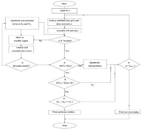
Flow chart of improved move limit with SLP is shown in the figure 4.1

Figure 4.1: Flow chart for improved move limit of SLP

5. INTRODUCTION TO OPTIMIZER

Optimizer is built on bases of sequential linear programming with improved move limit method consist of five subroutines, namely FUNCT, DERIV, SIMPLX, QUADIN and STEER with a analyzer subroutine called PROBLM. All the subroutines perform a unique and specific purpose.

5.1 Optimization of Precast Post-tensioned Concrete I-Girder Bridge

After the mathematical formulation of optimization problem, design program is developed and tested. Next step is to test the optimizer and connect the design program to optimizer. In this problem detailed study on process of Optimization of Precast Post-tensioned Concrete I-Girder Bridge is carried for span 30m with carriageway width of 7.5m, and M40 grade of concrete and Fe415 grade of steel.

 No of variables = 5

 No of constraints = 10

 Initial move limits = 0.1,0.1,0.1,0.1,0.1

 Lower limits on variables = 2.0,1.0,0.25,0.5,0.3

 Upper limit = 3.0,2.0,1.0,2.0,1.0

 Step length for calculating derivatives = 0.05

 Maximum number of function evaluation = 10000

 Maximum number of derivative evaluation = 1000

(5)

[image:5.595.32.289.208.595.2]

 Design program developed is connected to sequential linear programming based optimizer with the inputs as mentioned. Optimizer proceeded for number of function and derivative evaluation till the optimum point is reached. Using M40 grade concrete and Fe415 steel optimization is carried out for 30 m span.

Table 5.1: Progress of optimizer for precast post-tensioned concrete I-girder problem.

Where,

X1 = Over all depth of girder. X2 = Breadth of top flange. X3 = Depth of top flange. X4 = Breadth of top flange. X5 = Depth of bottom flange.

Figure 5.1: Variation of objective function with subsequent iterations

Table 5.2: Comparison of Optimum variables from various starting points

SI.NO Starting points Optimum points X1 X2 X3 X4 X5 X1 X2 X3 X4 X5 1 1.8 1.2 0.25 0.50 0.30 1.72 1.05 0.26 0.40 0.15 2 2.0 1.2 0.25 0.50 0.30 1.74 0.91 0.30 0.40 0.12 3 2.3 1.2 0.25 0.50 0.30 1.75 0.90 0.29 0.40 0.12 4 2.4 1.2 0.25 0.50 0.30 1.75 0.90 0.29 0.40 0.12 5 1.8 1.2 0.25 0.40 0.30 1.72 1.05 0.26 0.40 0.16 6 2.0 1.0 0.25 0.40 0.40 1.83 0.87 0.26 0.40 0.22

From the Table 5.2 it is clear that even though the problem was started with different starting points it resulting in almost same optimum points. Hence we can say that the global optimum is reached.

6. Results and Discussion

6.1 Effect of change in grade of concrete and steel.

[image:5.595.301.556.294.579.2]

Cost of the structure will be affected by grade of the concrete as well as steel. In this section effect of change in grade of the concrete and on optimum variables and cost of the structure is discussed. Following table gives for carriageway width of 7.5m.

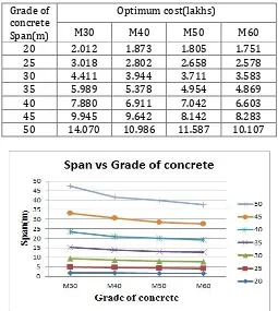
Table 6.1: Variation of optimum cost with change in grade of concrete.

Grade of concrete Span(m)

Optimum cost(lakhs)

M30 M40 M50 M60

20 2.012 1.873 1.805 1.751 25 3.018 2.802 2.658 2.578 30 4.411 3.944 3.711 3.583 35 5.989 5.378 4.954 4.869 40 7.880 6.911 7.042 6.603 45 9.945 9.642 8.142 8.283 50 14.070 10.986 11.587 10.107

Figure 6.1 Effect of concrete grade with span on cost By referring to table 6.1

 Total cost of the structure increases with increase in grade of concrete and span.

6.2

Cost ratio :

Cost ratio is defined as ratio of cost of unit volume of steel to the cost of unit volume of concrete. Cost of steel and concrete vary with time, hence parametric study is carried out for different cost ratios.

Study is carried out for carriageway width of 7.5m. Following are the inputs for each cost ratio.

Iteration No X1 X2 X3 X4 X5 Obj.fun(lakhs) Initial point 2.00 1.20 0.25 0.50 0.30 4.112

(6)

 Characteristics strength of concrete = 40 N/mm2

 Characteristics strength of steel = 500 N/mm2

 Span = 30m

[image:6.595.308.556.90.233.2]

Parametric study is conducted for different cost ratios, various span and grade of concrete and steel as follows.

Table 6.2: Optimum points for different cost ratios

Cost

ratio X1 Optimum design variables X2 X3 X4 X5 50 1.702 0.925 0.307 0.400 0.120 60 1.703 0.925 0.307 0.400 0.120 70 1.701 0.924 0.307 0.400 0.120 80 1.679 0.902 0.332 0.400 0.120 90 1.679 0.902 0.332 0.400 0.120 100 1.679 0.902 0.332 0.400 0.120 59.05 1.702 0.925 0.307 0.400 0.120

From table 6.2 it is clear that the variations in the design variables for different cost ratio between 50 to 100 is least (negligible). Optimum values for various span between 20m to 50m and for carriageway width of 7.5m are given bellow.

Table 6.3: Variation of optimum points with span

Span

(m) X1 Optimum design variables X2 X3 X4 X5 20 1.403 0.909 0.130 0.400 0.120 25 1.531 0.819 0.287 0.400 0.120 30 1.749 0.863 0.310 0.400 0.120 35 2.228 0.791 0.280 0.400 0.120 40 2.394 0.804 0.356 0.405 0.229 45 2.526 1.106 0.311 0.400 0.255 50 2.472 1.166 0.453 0.400 0.120

i)

Span has greater influence on design variable X1, as the span increases correspondingly depth also increases.

ii)

Span has slight influence on X2, i.e., as the span increases correspondingly X2 also increases.

iii)

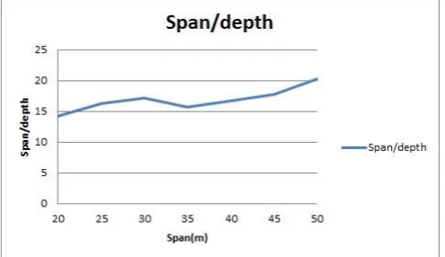
Span has least influence on other design variables (X3, X4, X5).

Table 6.4: Variation of depth with span

Span

(m) Depth (X1) (m) Span/Depth

20 1.403 14.26

25 1.531 16.33

30 1.749 17.15

35 2.228 15.71

40 2.394 16.71

45 2.526 17.81

50 2.472 20.23

Figure 6.2: Variation of depth with span

From the fig:6.2 it is clear that, Span has influence on depth of girder, i.e., as span increase depth of girder also increases, therefore span by depth ratio increases with increases with span. Variation of various ratios of design variables with span, for carriageway width of 7.5m are shown in the table below.

Table 6.5: Variation of various ratios of design variables with span

Span

(m) Optimum design variables Ratios

X1 X2 X3 X4 X5 X2/X3 X4/X5 X1/X2 X2/X4 X1/X4 20 1.40 0.91 0.13 0.40 0.12 6.99 3.33 1.54 2.27 3.51 25 1.53 0.82 0.29 0.40 0.12 2.85 3.33 1.87 2.05 3.83 30 1.75 0.86 0.31 0.40 0.12 2.78 3.33 2.03 2.16 4.37 35 2.23 0.79 0.28 0.40 0.12 2.83 3.33 2.82 1.98 557 40 2.39 0.81 0.36 0.40 0.23 2.20 1.75 2.98 2.01 5.99 45 2.53 1.11 0.31 0.41 0.26 3.56 1.59 2.28 2.73 6.24 50 2.47 1.17 0.45 0.40 0.12 2.57 3.33 2.12 2.92 6.18

From table 6.5 the following comments are made,

 The ratio X2/X3 with span remains constant (=2.8) for span between 25m to 35m.

 The ratio X2/X3 is least (=2.2) for span of 40m.  The ratio X4/X5 remains constants for span 20m to

35m.

 There is increase in the depth of bottom flange for span between 35m to 45m, which intern there is decrease in the ratio.

 In general, it is minimum requirements to be provided for various spans between 20m to 50m.

 For span between 20m to 40m, there is a less change in the X2/X4 remains constant.

 For spans greater then 40m, the X2/X4 ratio increases.

[image:6.595.36.281.188.308.2]

(7)

increases.

7. Conclusion

 Optimization of PSC I-girder is done by using sequential linear programming with improved move limit method.

 For span of 30m, carriageway width of 7.5m, fck = 40N/mm2_{and fy= 415N/mm}2_{, the various optimum}

values are,

a. Span by depth ratio is 17.271.

b. Top flange width by depth of top flange is 3.047.

c. Bottom flange width by depth of bottom flange is 3.333.

d. Top flange width by bottom flange width is 2.263.

 For any cost ratio between 50-100, Cost ratio does not influence much on the design variables.  It is recommended to use M30 or M40 grade

concrete for 20m to 30m span & M40 for 30m to 40m span, and M50 or M60 for 40m to 50m span.

 Following recommendation are also made, for carriageway width of 7.5m.

a. For any span between 25m to 35m, the ratio of top flange width to depth of top flange is 2.8.

b. For any span between 20m to 35m, the ratio of bottom flange width to depth of bottom flange is 3.33.

c. For any span between 25m to 40m, the ratio of top flange width to bottom flange width is 2.1.

8. Reference

1. Is:456-2000, Plain And Reinforced Concrete Code Of Practice, Bureau Of Indian Standards, New Delhi. 2. Irc:6-2014 Standard Specifications And Code Of

Practice For Road Bridges Section:Ii Loads And Stresses (Fourth Revision).

3. Irc:21-2000 Standard Specifications And Code Of Practice For Road Bridges Section:Iii Cement Concrete(Plain And Reinforced) (Third Revision). 4. Irc:18-2000 Design Criteria For Prestressed

Concrete Road Bridges(Post-Tensioned Concrete) (Third Revision).

5. Krinshna Raju .N., (2013) Prestressed Concrete, Tata Mccgrahil 5th Edition 2013.

6. Jagadeesh T. R., Jayaram M.A. (2012) Design Of Bridge Structures,Phi Learning Private Limited Second Edition 2012.

7. Bhavikatti S. S., "Fundamentals Of Optimum Design In Engineering",2nd_{Edition, New Academic Science}

Limited London, 2008.

8. Rao S. S., "Engineering Optimization Theory And Practice", 4th Edition, John Wiley And Sons Inc, 2009.

9. Samer Barakat, Ali Salem Al Harthy And Aouf R. Thamer Department Of Civil Emgineering, University Of Sharjah, Uae. Pakistan Journal Of Information And Technology 1(2):193-201, 2002. 10. Bhawar P.D, Wakchaure M.R, Nagare P.N

Optimization Of Pre-Stressed Concrete Girder, International Journal Of Research In Engineering And Technology (Ijret) Eissn:2319-1163, Volume: 04 Issue:03 /Mar-2015.

11. Mamoun Alqedra, Mohammed Arafa And Mohammed Ismail. Depart- Ment Of Civil Engineering,The Islamic University Of Gaza Palestine. Journal Of Artical Intelligence 4(1):76-88,2011 Issn 1994-5450 / Doi: 10.3923/Jai.2011.76.88.

12. Schedule Of Rates 2016-2017 Public Works, Ports & Inland Water Transport Department, North Zone, Dharwad.

Author Profile:

Prakash D. Mantur received the B.E. degrees in Civil Engineering from K.L.E. Institute of Technology Gokul, Hubballi, Karnataka in 2015, presently pursuing his masters in structure from K.L.E Technological University Hubballi, Karnataka(2015-2017).

Optimization of Precast Post tensioned Concrete I Girder Bridge