TRAINING AND DEVELOPMENT OFARTIFICIAL NEURAL NETWORK MODELS: SINGLE LAYER FEEDFORWARD AND MULTI LAYER FEEDFORWARD NEURAL NETWORK

(1)

ISSN: 1992-8645 www.jatit.org E-ISSN: 1817-3195

AFFINITY PROPAGATION AND RFM-MODEL FOR

CRM’S DATA ANALYSIS

1

E.S. MARGIANTI, 2R. REFIANTI, 3A.B. MUTIARA, 4K. NUZULINA

1

Prof., Faculty of Economics, Gunadarma University, Indonesia 2

Asst.Prof., Faculty of Computer Science and Information Technology, Gunadarma University, Indonesia 3

Prof., Faculty of Computer Science and Information Technology, Gunadarma University, Indonesia 4

Alumni, Graduate Program in Information System, Gunadarma University, Indonesia

E-mail: [email protected], 1,2{rina,[email protected], 3

[email protected]

ABSTRACT

The number of existing competition between companies make a company does not only focus on product development, but also in relation to customers. Customer Relationship Management (CRM) is a strategy to manage and maintain relationships with customers as well as an attempt to determine the wants and needs of customers. The analysis needs to produce the information on which customers are valuable or not. This will allow companies to implement efficient and effective measures to be loyal customers. This research is a data mining process with the method used is clustering by Affinity Propagation and Recency Frequency and Monetary (RFM) model on 1.000 Customer data. Distance method used on Affinity Propagation algorithm is Euclidean Distance and Manhattan Distance. Application was built using MATLAB to facilitate companies to analyze customer transaction data. From 1.000 customer data it generates 51 clusters. The best results if used Euclidean distance with preference median or Manhattan distance with preference minimum. The results of the clustering process is analyzed using comparison of RFM model and divide customer into eight type of customer and then into three groups. The results of customer segmentation are Most Valuable Customer 3.7%, Most Growable Customer 26.3% and Below Zero Customer 70%.

Keywords: Affinity Propagation, CRM, RFM, Clustering, Euclidean Distance, Manhattan Distance

1.

INTRODUCTION

A company can’t exist without the presence of customers. Different behavior of customer shopping and increasingly fierce competition makes the customer becomes important to be maintained. This is done so that the customer will always be loyal to the company. Loyalty is a form behavior of units to make a purchase decision continuously commodity or services of a company that is chosen [2]. Therefore, the company is not only focus on develop products that are offered, but also the direction of service and relationships to the customer.

Companies need the appropriate strategy so make easy to get customer loyalty. A strategy to manage and maintain relationships with customers as well as an attempt to determine the wants and needs of customers is also called Customer Relationship Management (CRM) [1]. Customer Relationship

Management is the process of modifying customer behavior from time to time and learn from each interaction, change, taking care of customers, and strengthen ties customers with corporate. CRM aims to know the customers and establish a good relationship to get customers, retain and develop customer into a valuable or beneficial customer. Application of CRM will make profits both for customers and the company.

(2)

ISSN: 1992-8645 www.jatit.org E-ISSN: 1817-3195 Data mining is analysis of survey data sets to find

unsuspected relationships and summarize the data in a different way than before, which is understandable and useful to the data owner. Various strategies can be used in the data mining process.

In this research, data mining proses within the method of clustering. One of the clustering algorithm is an algorithm that is introduced by Frey and Dueck, known as Affinity Propagation Algorithm [3].

Affinity Propagation is an algorithm that identifies exemplar between data points and formed a group of data points at around exemplar. Affinity Propagation consider all the data points as a candidate and then the real-value messages exchanged between the data points to the best exemplar [7,8].

This research then analysis of RFM models for Customer Relationship Management (RFM). This method is common method used in analyzing customer transaction data. RFM model is composed of Recency, Frequency, Monetary. RFM is a model to determine customer segmentation based on the span of the last transaction made by customers (Recency), the total amount or the average transaction in the period (frequency), and the total number or the average customer transaction (Monetary).

Implementation of Affinity Propagation clustering algorithm combined RFM model aims to determine the pattern of the data contained in customer transaction and customer identification with customer segmentation. The purpose of customer segmentation process is to know the behavior of customers. It is vital to implement appropriate strategies in order to know valuable customers and profitable for the company.

2.

RESEARCH METHODOLOGY

2.1 Research Design

The design phase of the research is problem-solving strategies in data mining called Cross-Industry Standard Process for Data Mining (CRISP-DM)[6]. CRISP-DM is composed into six phases as follows:

The research design of this system encompasses the following activities:

1) Business Understanding Phase:

Understanding the business is phase to know stage

of business processes contained in a company. It aims to obtain or find patterns in data mining clustering method with more precise results. In this research, analyzed on Customer Relationship Management (CRM) is how relationships between companies and consumers based on the existing transaction data. Related with this, the company can customize an effective marketing strategy to customer.

2) Data Understanding: In this phase is

analyzing the data that define attributes that will be analyzed. The data used in this research is that the data derived from the datasets where there are four fields as shown in table 2.1. Attribute models of the field carried are Recency, Frequency, Monetary (RFM) and processed at the next stage of the data preparation phase.

(3)

[image:3.612.96.293.106.215.2]

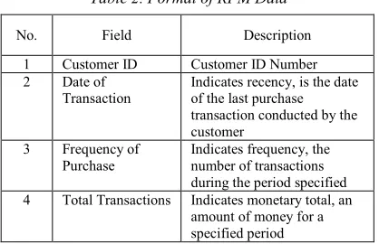
Table 2. Format of RFM Data

No. Field Description

1 Customer ID Customer ID Number

2 Date of

Transaction

Indicates recency, is the date of the last purchase transaction conducted by the customer

3 Frequency of Purchase

Indicates frequency, the number of transactions during the period specified 4 Total Transactions Indicates monetary total, an

amount of money for a specified period

Table 4. Parameter Table

Name Description

Distance method The method to compute the distance between two point are:

1: Euclidean Distance 2: Manhattan Distance

Preference Determines the preference by median or minimum

Table 5. Clustering Result Table

Table Column Description

Result 1st_column _{Customer ID Number} 2nd_column _{Cluster Number} 3rd_column _{Sum of customer each}

cluster 4th_column _{Recency Value}

5th_column _{Frequency Value}

6th column Monetary Value

3) Data Preparation: At this phase data

selection, preprocessing Phase /cleaning and data transformation will be done.

a) Data Selection: Selecting the data fields that used to next process at customer transaction data. Data transaction will process data cleaning with eliminate double data or invalid.

b) Data Preprocessing: The transaction data will be differentiated based on the specified attribute that is based on the model of RFM (Recency, Frequency, Monetary). RFM is a vulnerable time of the last transaction (Recency), the number of frequency customer transaction (Frequency) and the total number of transactions (Monetary).

c) Data Transformation: Grouping attributes into a single table for the segmentation process by using attributes Recency, Frequency, and Monetary. Existing data are compliant because the data is already in the form of an integer or number. The results of the data preparation phase are as follows:

4) Modeling Phase: At this phase, the process of

searching for patterns or means relationships at customer database transaction data by using a clustering algorithm, Affinity Propagation. Data were processed using comparison of the segmentation results by the average value of RFM. At this phase, the data that has been processed will

be clustering that divides customers into several clusters based on the pattern of relation was found.

In the data mining process with Affinity Propagation algorithm clustering method, there are four tables, namely the input table in Table 3., parameters table in Table 4., clustering results table in Table 5. and RFM analysis table in Table 6. as follows:

Table 3. Input Table

Table Column Description

Data 1st_column _{Customer ID Number}

2nd_column _{Indicates recency, is} the date of the last purchase transaction conducted by the customer

3rd_column _{Indicates frequency,} the number of transactions during the period specified 4th_column _{Indicates monetary}

total, an amount of money for a specified period

Table 1. Customer Transaction Data Tables

No. Field Description

1 Customer ID Customer ID Number

2 Date of

Transaction

Date of purchase transactions made by customers

3 Number Product Number of products purchased by customers

4 Total

Transactions

[image:3.612.93.302.509.644.2]

(4)

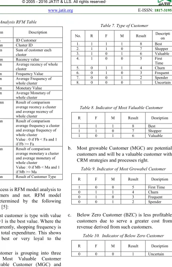
Table 7. Type of Customer

No. R F M Result Descripti

on

1. 1 1 1 8 Best

2. 1 1 0 7 Shopper

3. 1 0 1 6 Valuable

4. 1 0 0 5 First

Time

5. 0 1 1 4 Churn

6. 0 1 0 3 Frequent

7. 0 0 1 2 Spender

8. 0 0 0 1 Uncertain

Next clustering process is RFM model analysis to find valuable customers and not. RFM model analysis will be determined by the following conditions in Table 7. [5]:

In Table 7., the best customer is type with value are R=1, F=1 and M=1 is the best value. Where the customer shopping currently, shopping frequency is often with very large total expenditure. This shows that customers are best or very loyal to the company.

Eight types of customer is grouping into three categories namely Most Valuable Customer (MVC), Most Growable Customer (MGC) and Below Zero Customer (BZC). Here is an indicator of the type of customer [1]:

a. Most Valuable Customer (MVC) that customers who currently provide to the company profile.

b. Most growable Customer (MGC) are potential customers and will be a valuable customer with CRM strategies and processes right.

c. Below Zero Customer (BZC) is less profitable customers due to serve a greater cost from revenue derived from such customers.

5) Evaluation Phase: This phase is evaluation of

the modeling process used. Evaluation is used to evaluation the number of clusters and distribution of segmentation result. Also check customer categories are in accordance with the understanding bussiness.

6) Deployment Phase: This phase is making data

mining applications using MATLAB to generate a report in the form of visualization that allows users to see the results of segmentation. This will facilitate in making appopriate strategy in each type

Table 10. Indicator of Below Zero Customer

R F M Result Desription

0 0 0 1 Uncertain

Table 9. Indicator of Most Growabel Customer

1 0 0 5 First Time

0 1 1 4 Churn

0 1 0 3 Frequent

0 0 1 2 Spender

Table 8. Indicator of Most Valuable Customer

1 1 1 8 Best

1 1 0 7 Shopper

[image:4.612.177.522.61.595.2]

1 0 1 6 Valuable

Table 6. Analysis RFM Table

Table Coloumn Description

Result 1st coloumn ID Customer

2nd coloumn Cluster ID

3rd coloumn Sum of customer each cluster

4th coloumn Recency value

5th coloumn Average recency of whole cluster

6th coloumn Frequency Value 7th coloumn Average Frequency of

whole cluster

8th coloumn Monetary Value

9th coloumn Average Monetary of whole cluster 10th coloumn Result of comparison

average recency a cluster and average recency of whole cluster 11th_coloumn _{Result of comparison}

average frequency a cluster and average frequency of whole cluster

Value : 0 if Fb < Fa and 1 if Fb >= Fa

12th_coloumn _{Result of comparison} average monetary a cluster and average monetary of whole cluster

Value : 0 if Mb < Ma and 1 if Mb >= Ma

(5)

ISSN: 1992-8645 www.jatit.org E-ISSN: 1817-3195 of customer so that the customer will be loyal to the

company.

2.2 Affinity Propagation and RFM Model

The process of data mining is the clustering using Affinity Propagation algorithm and RFM model analysis. Here is a process that is performed in finding patterns in customer transaction data.

Step 1. Input, Process and Output

Data processing consists of three fields namely Recency, Frequency and Monetary.

Step 2. Clustering with Affinity Propagation [3][7,8]

Affinity Propagation will analyze and calculate the distance method by Euclidean Distance or Manhattan Distance and create similarity matrix.

{

1,..., } )

, (

{s i j _ijε N (1)

Determine the preference of the similarity matrix is formed by calculating median or minimum.

0 ) , ( : , ) ,

(k k = p∀i k a i k =

s (2)

The initial availability value is a zero matrix. This value is availability value at early step to calculate availability value in the first iteration.

0 ) , ( : , =

∀ik aik (3)

The algorithm will calculate responsibility value on the data matrix. The value of responsibility is a message that sent data point i to the data point k to be a candidate exemplar for the data point i. The formula for determining responsibility matrix is as follows: )} , ( ) , ( max{ ) , ( ) ,

(ik si k aik sik

r ← + (4)

Calculation of availability value contains the message sent by the candidate exemplar to the data points. Availability value of a data point will consider the value of the data points the other to be the exemplar for the data point. Determination of the data points to the cluster members or exemplar based on the values of responsibility and availability. The formula for determining the value of the next iteration matrix availability are as follows:

∑

=

← r i k fork i

k k

a( , ) max{0, (, )},

(5) i fork k i r k k r k i

a(, )←min{0, ( , )+

∑

max{0, (, )}, ≠ (6)

Determining the convergent value for Affinity Propagation clustering. Value of availability and responsibility will send messages. Availability send

messages to the data point i on how good the data point k to be a candidate exemplar for the data point i. Responsibility sending a data message point i to the candidate k exemplar of how well the data point k to be a candidate exemplar for the data point i. The condition is repeated until getting value convergent. Convergent is a state when the value is not changed after a few iterations. The formula for determining the convergence conditions as follows:

) , ( ) , ( ) ,

(i k r i k a i k

c ← + (7)

Step 3. RFM Analysis

Analysis RFM based on the clustering of Affinity Propagation algorithm.

a. Calculate the average value of the Recency, Frequency and Monetary in each cluster. b. Calculate the average value Recency in

overall cluster, the average value of the overall frequency in the cluster, and the average value of the Monetary overall in the cluster.

c. Comparing the average value of the cluster with the overall average. If overall average is larger than average in a cluster data so value is 1. If it is smaller than the data in a cluster then value is 0 which indicates the average of data in the cluster is smaller than the overall average.

Based on these results it can be seen how the pattern when shopping, frequency and monetary of customers in each cluster.

Step 4. Prediction

a. Determine the category of customer based on the value of RFM and the average RFM b. Recommendation valuable customers, customer growth with the right strategy and customer are less profitable for the company.

3.

IMPLEMENTATION AND RESULT

3.1 Clustering with Affinity Propagation

Affinity Propagation is a message-passing algorithms and simultaneously considering all the data points as an exemplar candidate to get the value of convergence.

(6)

ISSN: 1992-8645 www.jatit.org E-ISSN: 1817-3195 matrix based on the calculation of the distance

between the negative values of the data point. Distance method using Euclidean distance and Manhattan distance.

Preference value is determination of diagonal value in the matrix. Preference value set number of clusters found by the Affinity Propagation. Small preference value produces smaller clusters. An example calculation similarity between customer number 01 and 02 customers is calculation by euclidean distance such as

(

533−522

)

2+

(

1−2

)

2+

(

12−89

)

2= 6051=77.788

=

d

Diagonal values in the similarity matrix is determined in two ways are the median or middle value of the matrix and minimum or smallest value of the matrix. The data obtained preference median value is 223.4659 and the minimum is -4.4122e+003.

In the following calculations are used, resulting similarity matrix based methods euclidean distance with a median value of preference. Similarity matrix formed is as follows:

Figure 2. Similarity Matrix

The next process, the algorithm forming availability with zero matrix in the first iteration. Next is count the responsibility matrix of similarity. Here is a snippet of resulting responsibility matrix.

Figure 3. Responsibility Matrix

Furthermore, the value of availability between one point with other point are calculated. The next iteration will produce availability value as follows:

Figure 4. Availability Matrix

Value on availability and responsibility send messages to generate convergence value. Value on the similarity matrix will be turned into a positive. At iteration 379 no changes in value and are called state convergence.

Based on 1000 data obtained clustering results in the form of iteration, the number of clusters, the time duration of the process of clustering. Clustering based on data from 1000 customer that can be seen in Table 11. as follows:

3.2 Analysis RFM with RFM Model

The results of the transaction data were processed using Affinity Propagation algorithm will be analyzed by RFM models. RFM analysis aims to divide the customer based on the customer's behavior. RFM analysis is done by comparing data Mean Recency with Recency. Mean frequency with Frequency and Mean Monetary with the Monetary. Here is the result of RFM model comparison:

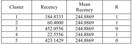
3.2.1 Recency and Mean Recency

[image:6.612.311.526.482.556.2]

In Table 12. are 5 of the 51 clusters of the 1000 data. The value of R=1 obtained pieces of 1,2,4 and the value R=0 obtained by clusters 3 and 5. R=0 indicates recency of data is smaller than the mean recency. R=1 shows the recency of data is greater than the mean recency. It shows that the cluster with the value of R= 1 is the customer who makes a purchase is recent of time period.

Table 12. Comparison of Recency and Mean Recency

Cluster Recency Mean

Recency R

1 184.8333 244.8869 1

2 60.4000 244.8869 1

3 452.0556 244.8869 0

4 22.5556 244.8869 1

5 423.1429 244.8869 0

Table 11. Clustering Result by Affinity Propagation Algorithm

Distance

Method Preference Sum

of Data

Itera-tion

Clu-ster Time

Euclidean Median 1000 379 51 26

Euclidean Minimum 1000 143 8 13

Manhattan Median 1000 377 51 26

(7)

3.2.2 Frequency and Mean Frequency

In Table 13. are 5 of the 51 clusters clustering results. Of the 15 clusters, the value of F = 1 are in the cluster while the other cluster 2,4,6 get a value of 0. F = 0 indicates the data frequency is smaller than the mean frequency. F = 1 shows the frequency of data is greater than the mean frequency. It shows that the cluster with the value of F = 1 is the customers who make purchases more frequently than the average purchase in the cluster.

3.2.3 Monetary and Mean Monetary

In Table 14. are 5 of the 51 clusters of the 1000 data. Based on the 5 clusters, the value of M = 1 are in the cluster 2,4 while the other cluster get a value of 0. M = 1 indicates the monetary data is smaller than the mean monetary. M = 1 shows the monetary data is greater than the mean monetary. It shows that the cluster with the value of M = 1 is total customer transactions greater than average total transactions in overall cluster. These results integrated and produce value as follows:

In Table 15. the best value is the value of R=1, F=1 and F value with the value of 1 is the best value. It show that the customer is recently shopping, shopping frequency is often with total

transactions very large. This shows that customers are very valuable to the company.

In Table 16., 5 of the 51 clusters from 1.000 customer data generate customer types as follows:

In RFM analysis on 1000 data, there are 5 customer types: type 1,2,5,6 and 8. The number of customers of each type is Uncertain as much 700 customers, Spender as much 2 customers, First time as much 261 customers, and Valuable 2 customers and Best 8 customers.

3.3 Testing Result

The test result is a process to know about success in achieving the goal of this research. The data used in this research is 1.000 customers data in a period of one year. Clustering result on the data RFM is done by comparing the amount of data and iteration of the clustering time. Clustering results with the model RFM will segmentation process by comparing the average of each cluster with the overall average on every attribute RFM models.

3.3.1 Clustering with Affinity Propagation Algorithm

Clustering process using Affinity Propagation algorithm is tested by determining the distance and method of preference. Distance method used is Euclidean Distance and Manhattan Distance. Data used 1.000 customer data. The trial clustering with Affinity Propagation algorithm is divided into the following four conditions:

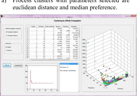
[image:7.612.87.301.363.437.2]

a) Process clusters with parameters selected are euclidean distance and median preference.

Figure 5. Page Clustering AP With Euclidean & Preference Median

Distance

Method Preference

Sum of

Data Cluster

Customer Type

Euclidean Median 1000 51 1,2,5,6,8

[image:7.612.313.535.548.704.2]

Euclidean Minimum 1000 8 1,5,8

Cluster R F M Result Description

1 1 0 0 5 First time

2 1 1 1 8 Best

3 0 0 0 1 Uncertain

4 1 1 1 8 Best

5 0 0 0 1 Uncertain

Table 14. Comparison of Monetary and Mean Monetary

Cluster Monetary Mean

Monetary M

1 374.8333 489.6050 0

2 1.0714e+03 489.6050 1

3 96.3889 489.6050 0

4 572.4444 489.6050 1

5 52.7857 489.6050 0

Table 13. Comparison of Frequency and Mean Frequency

Cluster Frequency Mean

Frequency F

1 8 9.2970 0

2 21 9.2970 1

3 2.5000 9.2970 0

4 17.1111 9.2970 1

[image:7.612.88.298.577.668.2]

(8)

ISSN: 1992-8645 www.jatit.org E-ISSN: 1817-3195 Affinity Propagation clustering algorithms

include as much as 379 times the number of iterations, the number of clusters as many as 51 and iteration time for 25 seconds.

[image:8.612.306.531.75.234.2]

b) Process clusters with parameters selected are euclidean distance and preference minimum

Figure 6. Page Clustering AP With Euclidean & Preference Minimum

The results of Affinity Propagation clustering algorithms include as much as 143 times the number of iterations of the iteration, the number of clusters as many as 8 and iteration time for 12 seconds.

c) Process clusters with parameters selected are manhattan distance and preference median.

Figure 7. Page Clustering AP With Manhattan & Preference Median

The results of Affinity Propagation clustering algorithms include as much as 377 times the number of iterations of the iteration, the number of clusters 51 and iteration time for 25 seconds

d) Process clusters with parameters selected are manhattan distance and preference minimum

Figure 8. Page Clustering AP With Manhattan & Preference Minimum

The results of Affinity Propagation clustering algorithms include as much as 99 times the number of iterations of the iteration, the number of clusters 8 and iteration time for 11 seconds.

[image:8.612.89.305.140.326.2]

Testing do at 600 until 1.000 data obtained clustering results in the form of iteration, the number of clusters and clustering process time. Comparison of clustering result with a median preference can be seen in Table 17. Comparison of clustering result with preference minimum can be seen in Table 18.

Table 17. Comparison Clustering Result with Preference Median

No Distance _Method Pre-_ference Sum of Data

Itera tion

Clu ster Time

1. Euclidean Median 600 358 35 8.6

Manhattan Median 385 36 9.2

2. Euclidean Median 700 360 39 11

Manhattan Median 364 41 13

[image:8.612.102.481.399.568.2]

(9)

3.4 Analysis of Customer Type

Clustering and RFM analysis in this research was conducted on 1.000 data. Clustering result with Affinity Propagation algorithm is not much different even though the distance method is Euclidean distance and Manhattan distance.

[image:9.612.313.527.369.437.2]

Results from RFM analysis and Affinity Propagation algorithm with euclidean distance method is as follows:

Figure 9. RFM Analysis From 1000 Data With Euclidean Distance

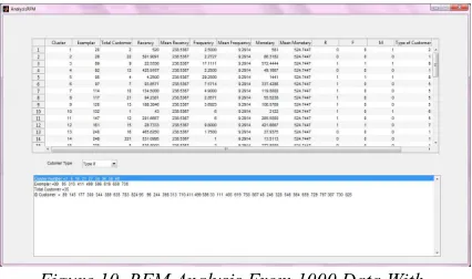
Results from RFM analysis and Affinity Propagation algorithm with manhattan distance method is as follows:

Figure 10. RFM Analysis From 1000 Data With Manhattan Distance

[image:9.612.90.301.387.526.2]

Both methods produce customers type such as Type 1, Type 2, Type 5, Type 6 and Type 8. Here difference the number of customers on the customer type that is obtained can be seen in Figure 11.

Figure 11. RFM Analysis Result

In Type 1, Euclidean Distance has 700 customers but Manhattan Distance have 721 customers. In Type 5 Euclidean Distance have 261 customers but Manhattan Distance have 240 customers. On the other types: type 2, type 6 and type 8 have the same number of customers. Type 2 has 2 customers, type 6 has 2 customers and Type 8 has 35 customers who belong to that type.

Type 1 is the type of customer who has a tendency to have not shopped, rarely make purchases and total transactions are small. In the dataset found 700 customers or 721 customers. This can be seen in example from 3 customers spending included in type 1 as follows:

Type 2 is the type of customer that has a tendency rather long shopping, purchases with a total frequency of rare and total transactions are big. In dataset found 2 customers, it can be seen at the example of 2 customers that included in type 2 as follows:

Type 5 is the type of customer that has recently of shopping, rarely make purchases and total transactions are small. In the dataset found 261 or 240 customers. This can be seen in example of 2 customers that can be seen as follows:

Table 20. Customer Type 2

Customer

ID Recency Frequency Monetary

20 516 2 653

457 524 3 509

Customer

12 533 1 57

15 533 1 53

[image:9.612.313.525.534.581.2]

57 533 1 58

Table 18. Comparison Clustering Result with Preference Minimum

No Distance Method

Pre-ference

Sum of Data

Itera tion

Clu ster

Ti me

1. Euclidean Minimum 600 125 5 3.8

Manhattan Minimum 89 5 3.4

5. Euclidean Minimum 1000 143 8 13

[image:9.612.90.303.580.706.2]

(10)

Type 6 is the type of customer who has long not to shop, often make a purchase, but with small total transactions. Found 2 customers dataset. This can be seen in example of 2 customers that can be seen as follows:

Type 8 is a type of new customers who have recency to shopping, often make purchases and transactions are large total. In the dataset found 8 customers. This can be seen in example of 2 customers that can be seen as follows:

[image:10.612.319.520.158.288.2]

The presentation results of customer types can be seen in Figure 12.:

Figure 12. Graphic of Customer Type

Customer Type Divided to be 5 there are type 1 which is the type of customer that is uncertain. Total customer in type 1 is 70% of the 1.000 data. Type 8 is the best customer as much as 3.7%. Type 5 is the type of first-time customers as much as 26.3%. Type 2 is the type of spender as much as

0.2% and Type 6 is the type valuable customer as much as 0.2%. Based on these data the customer regrouped into three. Most Valuable Customer, Most Growable Customer and Below Zero Customer as follows:

Figure 13. Graphic of Customer Category

Based on 1000 data, the result of customer's category are Most Valuable Customer 3.7% as much 37 customers, Most Growable Customer 26.3% as much 263 customers and Below Zero Customers 70% from data as much 700 customers.

4.

CONCLUSION

The conclusion of this research is as follows:

Affinity Propagation algorithm and using RFM model can find out more details about the types of customer to perform effective strategies.

The result of the comparison is the best result if used Euclidean distance with preference median and Manhattan distance with preference minimum.

Based on 1.000 data by Euclidean distance and preference median, the result of the customer's category are the Most Valuable Customer 3.7% or as many as 37 customers, Most Growable Customer 26.3% as much 263 customers and Below Zero Customers 70% of the data or as many as 700 customers.

REFERENCES

[1] Atmaja and S. Lukas, “Manajemen Keuangan”, Buku 1, penerbit Andi, Yogyakarta, 2001. [2] J. Griffin, “Customer Loyalty, Menumbuhkan

dan Mempertahankan Kesetiaan Pelanggan”, Jakarta: Erlangga, 2005.

[image:10.612.93.300.251.305.2]

[3] D. Delbert, “Affinity Propagation: Clustering Data by Passing Messages”, University of Toronto, 2009.

Customer

387 19 13 841

730 121 17 855

758 24 33 934

Customer

132 43 6 2122

548 43 7 1970

Table 21.Customer Type 5

Customer

53 50 6 86

78 61 2 95

[image:10.612.89.302.385.444.2] [image:10.612.99.290.480.649.2]

(11)

ISSN: 1992-8645 www.jatit.org E-ISSN: 1817-3195 [4] Fader and Hardie, “Repeat Sales Forecasting

At CDNOW: A case study”, 2001.

[5] L. Duen-Ren and S. Ya-Yueh, “Integrating AHP and Data Mining for Product Recommendation Based on Customer Lifetime Value”. Taiwan, 2005, pp. 387-400.

[6] D.L. Olson and D. Delen, “Advanced Data Mining Techniques”, New York: Springer, 2008, pp. 9-35. ISBN: 978-3-540-76916-3. [7] R.Refianti, A.B.Mutiara, A. Juarna, and S.N.

Ikhsan, “Analysis and Implementation of Algorithm Clustering Affinity Propagation and K-Means At Data Student Based On GPA and Duration of Bachelor Thesis Completion”, Journal of Theoretical and Applied Information Technology, Vol. 35 No. 1, 2012, pp. 69-76. [8] S. Jatmiko, R. Refianti, A.B. Mutiara, and R.