SRC RR 91 pdf

91

An Old-Fashioned Recipe for

Real Time

Mart´ın Abadi and Leslie Lamport

Systems Research Center

DEC’s business and technology objectives require a strong research program. The Systems Research Center (SRC) and three other research laboratories are committed to filling that need.

SRC began recruiting its first research scientists in l984—their charter, to advance the state of knowledge in all aspects of computer systems research. Our current work includes exploring high-performance personal computing, distributed com-puting, programming environments, system modelling techniques, specification technology, and tightly-coupled multiprocessors.

Our approach to both hardware and software research is to create and use real systems so that we can investigate their properties fully. Complex systems cannot be evaluated solely in the abstract. Based on this belief, our strategy is to demonstrate the technical and practical feasibility of our ideas by building prototypes and using them as daily tools. The experience we gain is useful in the short term in enabling us to refine our designs, and invaluable in the long term in helping us to advance the state of knowledge about those systems. Most of the major advances in information systems have come through this strategy, including time-sharing, the ArpaNet, and distributed personal computing.

SRC also performs work of a more mathematical flavor which complements our systems research. Some of this work is in established fields of theoretical computer science, such as the analysis of algorithms, computational geometry, and logics of programming. The rest of this work explores new ground motivated by problems that arise in our systems research.

DEC has a strong commitment to communicating the results and experience gained through pursuing these activities. The Company values the improved understanding that comes with exposing and testing our ideas within the research community. SRC will therefore report results in conferences, in professional journals, and in our research report series. We will seek users for our prototype systems among those with whom we have common research interests, and we will encourage collaboration with university researchers.

An Old-Fashioned Recipe for Real Time

Mart´ın Abadi and Leslie Lamport

c

Digital Equipment Corporation 1992

Authors’ Abstract

Contents

1 Introduction 1

2 Closed Systems 2

2.1 The Lossy-Queue Example: : : : : : : : : : : : : : : : : : : : : 3 2.2 The Semantics of TLA : : : : : : : : : : : : : : : : : : : : : : : 7 2.3 Safety and Fairness: : : : : : : : : : : : : : : : : : : : : : : : : 8 2.4 History-Determined Variables : : : : : : : : : : : : : : : : : : : 10

3 Real-Time Closed Systems 11

3.1 Time and Timers : : : : : : : : : : : : : : : : : : : : : : : : : : 11 3.2 Reasoning About Time : : : : : : : : : : : : : : : : : : : : : : : 14 3.3 The NonZeno Condition : : : : : : : : : : : : : : : : : : : : : : 17 3.4 An Example: Fischer’s Protocol : : : : : : : : : : : : : : : : : : 21

4 Open Systems 24

4.1 Receptiveness and Realizability : : : : : : : : : : : : : : : : : : 24 4.2 The FOperator : : : : : : : : : : : : : : : : : : : : : : : : : : 25 4.3 Proving Machine Realizability : : : : : : : : : : : : : : : : : : : 25 4.4 Reduction to Closed Systems: : : : : : : : : : : : : : : : : : : : 26 4.5 Composition : : : : : : : : : : : : : : : : : : : : : : : : : : : : 27

5 Real-Time Open Systems 27

5.1 A Paradox : : : : : : : : : : : : : : : : : : : : : : : : : : : : : 28 5.2 Timing Constraints in General : : : : : : : : : : : : : : : : : : : 31

6 Conclusion 32

A Definitions 35 A.1 States and Behaviors : : : : : : : : : : : : : : : : : : : : : : : : 35 A.2 Predicates and Actions : : : : : : : : : : : : : : : : : : : : : : : 35 A.3 Properties : : : : : : : : : : : : : : : : : : : : : : : : : : : : : 36 A.4 Closure and Safety : : : : : : : : : : : : : : : : : : : : : : : : : 36 A.5 Realizability : : : : : : : : : : : : : : : : : : : : : : : : : : : : 36

B Proofs 37

B.1 Proof Notation : : : : : : : : : : : : : : : : : : : : : : : : : : : 37 B.2 Proof of Proposition 2 : : : : : : : : : : : : : : : : : : : : : : : 38 B.3 Proof of Proposition 3 : : : : : : : : : : : : : : : : : : : : : : : 38 B.4 Two Lemmas About Machine-Realizability : : : : : : : : : : : : 39 B.5 Proof of Proposition 4 : : : : : : : : : : : : : : : : : : : : : : : 40 B.6 Proof of Proposition 5 : : : : : : : : : : : : : : : : : : : : : : : 45 B.7 Proof of Theorem 4 : : : : : : : : : : : : : : : : : : : : : : : : 46 B.7.1 High-Level Proof of the Theorem : : : : : : : : : : : : : 47 B.7.2 Detailed Proof of the Theorem : : : : : : : : : : : : : : : 51

References 61

1

Introduction

A new class of systems is often viewed as an opportunity to invent a new semantics. A number of years ago, the new class was distributed systems. More recently, it has been real-time systems. The proliferation of new semantics may be fun for semanticists, but developing a practical method for reasoning formally about systems is a lot of work. It would be unfortunate if every new class of systems required inventing new semantics, along with proof rules, languages, and tools. Fortunately, no fundamental change to the old methods for specifying and reasoning about systems is needed for these new classes. It has long been known that the methods originally developed for shared-memory multiprocessing apply equally well to distributed systems [7, 11]. The first application we have seen of a clearly “off-the-shelf” method to a real-time algorithm was in 1983 [16], but there were probably earlier ones. Indeed, the “extension” of an existing temporal logic to real-time programs by Bernstein and Harter in 1981 [6] can be viewed as an application of that logic.

The old-fashioned methods handle real time by introducing a variable, which we call now, to represent time. This idea is so simple and obvious that it seems hardly worth writing about, except that few people appear to be aware that it works in practice. We therefore describe how to apply a conventional method to real-time systems.

Any formalism for reasoning about concurrent programs can be used to prove properties of real-time systems. However, in a conventional formalism based on a programming language, real-time assumptions are expressed by adding program operations that read and modify the variablenow. The result can be a complicated

program that is hard to understand and easy to get wrong. We take as our formalism TLA, the temporal logic of actions [13]. In TLA, programs and properties are rep-resented as logical formulas. A real-time program can be written as the conjunction of its untimed version, expressed in a standard way as a TLA formula, and its timing assumptions, expressed in terms of a few standard parameterized formulas. This separate specification of timing properties makes real-time specifications easier to write and understand.

the operations. Its correctness is proved by a conventional invariance argument. We also discuss two problems that arise when time is represented as a program variable—problems that seem to have received little attention—and present new solutions. The solutions are expressed in terms of TLA, but they can be applied to any formalism whose semantics is based on sequences of states or actions. The first problem is how to avoid the real-time programming version of Zeno’s paradox. If time becomes an ordinary program variable, then one can inadvertently write programs in which time behaves improperly. An obvious danger is deadlock, where time stops. A more insidious possibility is that time keeps advancing but is bounded, approaching closer and closer to some limit. One way to avoid such “Zeno” behaviors is to place an a priori lower bound on the duration of any action, but this can complicate the representation of some systems. We provide a more general and, we feel, a more natural solution.

The second problem is coping with the circularity that arises in open system spec-ifications. The specification of an open system asserts that it operates correctly under some assumptions on the system’s environment. A modular specification method requires a rule asserting that, if each component satisfies its specification, then it behaves correctly in concert with other components. This rule is circu-lar, because a component’s specification requires only that it behave correctly if its environment does, and its environment consists of all the other components. Despite its circularity, the rule is sound for specifications written in a particular style [1, 15, 17]. By examining an apparently paradoxical example, we discover how real-time specifications of open systems can be written in this style.

2

Closed Systems

We briefly review how to represent closed systems in TLA. A closed system is one that is self-contained and does not communicate with an environment. No one intentionally designs autistic systems; in a closed system, the environment is represented as part of the system. Open systems, in which the environment and system are separated, are discussed in Section 4.

-ibit ival

obit oval

q: : : :

last:

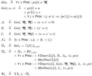
Figure 1: A simple queue.

Propositions and theorems are proved in the appendix.

2.1

The Lossy-Queue Example

We introduce TLA with the example of the lossy queue shown in Figure 1. The interface consists of two pairs of “wires”, each pair consisting of aval wire that

holds a message and a boolean-valuedbit wire. A message m is sent over a pair

of wires by setting theval wire to m and complementing the bit wire. Input to

the queue arrives on the wire pair.ival;ibit/, and output is sent on the wire pair

.oval;obit/. There is no acknowledgment protocol, so inputs are lost if they arrive faster than the queue processes them. The property guaranteed by this lossy queue is that the sequence of output messages is a subsequence of the sequence of input messages. In Section 3.1, we add timing constraints to rule out the possibility of lost messages.

A specification is a TLA formula 5 describing a set of allowed behaviors. A property P is also a TLA formula. The specification5satisfies property P iff

(if and only if) every behavior allowed by5is also allowed by P—that is, if5

impliesP. Similarly, a specification9 implements5iff every behavior allowed by9is also allowed by5, so implementation means implication.

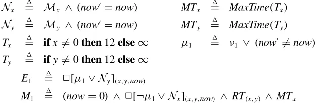
The specification of the lossy queue is a TLA formula that mentions the four variables ibit, obit, ival, and oval, as well as two internal variables: q, which

equals the sequence of messages received but not yet output; and last, which

equals the value ofibit for the last received message. (The variable last is used

to prevent the same message from being received twice.) These six variables are

flexible variables; their values can change during a behavior. We also introduce

InitQ D1 ^ ibit;obit2 ftrue;falseg ^ ival;oval2Msg

^ lastDibit

^ q D hhii

Inp D1 ^ ibit0 D :ibit

^ ival02Msg

^ .obit;oval;q;last/0_{D.obit;oval;q;last/}

EnQ D1 ^ last6Dibit

^ q0_{DqŽ hhivalii}

^ last0Dibit

^ .ibit;obit;ival;oval/0_D._ibit;_obit;_ival;_oval/

DeQ D1 ^ q 6D hhii

^ oval0DHead.q/

^ q0_DTail._q/

^ obit0D :obit

^ .ibit;ival;last/0_D._ibit;_ival;_last/

NQ

1

D Inp _ EnQ _ DeQ

v D1 .ibit;obit;ival;oval;q;last/

5Q

1

D InitQ ^ 2[NQ]v

8Q

1

D 9q;last :5Q

Figure 2: The TLA specification of a lossy queue.

throughout a behavior. We usually refer to flexible variables simply as variables, and to rigid variables asconstants.

The TLA specification is shown in Figure 2, using the following notation. A list of formulas, each prefaced by ^, denotes the conjunction of the formulas, and indentation is used to eliminate parentheses. The expressionhh iidenotes the empty sequence,hhmiidenotes the singleton sequence havingm as its one element,Ž

denotes concatenation,Head.¦/denotes the first element of¦, andTail.¦/denotes the sequence obtained by removing the first element of¦. The symbolD1 meansis defined to equal.

predicate asserts that the values of variablesibit and obit are arbitrary booleans, the

values ofival and oval are elements ofMsg, the values oflast and ibit are equal,

and the value ofq is the empty sequence.

Next is defined theaction Inp, which describes all state changes that represent the

sending of an input message. (Since this is the specification of a closed system, it includes the environment’sInp action.) The first conjunct, ibit0_{D :ibit, asserts that} the new value ofibit equals the complement of its old value. The second conjunct

asserts that the new value ofival is an element ofMsg. The third conjunct asserts that the value of the four-tuple.obit;oval;q;last/is unchanged; it is equivalent to the assertion that the value of each of the four variablesobit, oval, q, and last is

unchanged. The actionInp is always enabled, meaning that, in any state, a new

input message can be sent.

ActionEnQ represents the receipt of a message by the system. The first conjunct

asserts thatlast is not equal to ibit, so the message on the input wire has not yet been

received. The second conjunct asserts that the new value ofq equals the sequence

obtained by concatenating the old value ofival to the end of q’s old value. The third

conjunct asserts that the new value oflast equals the old value of ibit. The final

conjunct asserts that the values ofibit, obit, ival, and oval are unchanged. Action EnQ is enabled in a state iff the values of last and ibit in that state are unequal.

The actionDeQ represents the operation of removing a message from the head of q and sending it on the output wire. It is enabled iff the value of q is not the empty

sequence.

The actionNQ is the specification’snext-state relation. It describes all allowed changes to the queue system’s variables. Since the only allowed changes are the ones described by the actionsInp, EnQ, and DeQ, actionNQis the disjunction of those three actions.

In TLA specifications, it is convenient to give a name to the tuple of all relevant variables. Here, we call itv.

Formula5Qis the internal specification of the lossy queue—the formula specifying

all sequences of values that may be assumed by the queue’s six variables, including the internal variablesq and last. Its first conjunct asserts that InitQis true in the

initial state. Its second conjunct,2[NQ]v, asserts that every step is either anNQ step (a state change allowed byNQ) or else leavesv unchanged, meaning that it leaves all six variables unchanged.

Formula8Q is the actual specification, in which the internal variablesq and last

of values toq and last such that5Qis satisfied. The free variables of8Qareibit,

obit, ival, and oval, so8Qspecifies what sequences of values these four variables

can assume. All the preceding definitions just represent one possible way of structuring the definition of8Q; there are infinitely many ways to write formulas

that are equivalent to8Qand are therefore equivalent specifications.

TLA is an untyped logic; a variable may assume any value. Type correctness is expressed by the formula2T , where T is the predicate asserting that all relevant variables have values of the expected “types”. For the internal queue specification, the type-correctness predicate is

TQ D ^1 ibit;obit;last2 ftrue;falseg ^ ival;oval2Msg

^ q 2MsgŁ

(1)

whereMsgŁ _{is the set of finite sequences of messages. Type correctness of}5

Qis

asserted by the formula5Q )2TQ, which is easily proved [13]. Type correctness of8Qfollows from5Q)2TQby the usual rules for reasoning about quantifiers. Formulas5Qand8Qaresafety properties, meaning that they are satisfied by an

infinite behavior iff they are satisfied by every finite initial portion of the behav-ior. Safety properties allow behaviors in which a system performs properly for a while and then the values of all variables are frozen, never to change again. In asynchronous systems, such undesirable behaviors are ruled out by addingfairness

properties. We could strengthen our lossy-queue specification by conjoining the

weak fairness property WF_v.De Q/and thestrong fairness property SF_v.EnQ/to

5Q, obtaining

9q;last :.InitQ ^ 2[NQ]v ^ WFv.De Q/ ^ SFv.EnQ// (2)

Property WFv.De Q/asserts that if actionDeQ is enabled forever, then infinitely

manyDeQ steps must occur. This property implies that every message reaching

the queue is eventually output. Property SF_v.EnQ/ asserts that if actionEnQ is

enabled infinitely often, then infinitely manyEnQ steps must occur. It implies that

if infinitely many inputs are sent, then the queue must receive infinitely many of them. The formula (2) implies theliveness property [4] that an infinite number of

inputs produces an infinite number of outputs. This formula also implies the same safety properties as8Q. A formula such as (2), which is the conjunction of an

initial predicate, a term of the form2[A]f, and a fairness property, is said to be in

2.2

The Semantics of TLA

We begin with some definitions. We assume a set of constantvalues, and we let

[[F]] denote the semantic meaning of a formula F.

state A mapping from variables to values. We let s:x denote the value that state s

assigns to variablex .

state function An expression formed from variables, constants, and operators. The meaning of a state function is a mapping from states to values. For example,x C1 is a state function such that [[x C1]].s/equalss:x C1, for any states.

predicate A boolean-valued state function, such as x> yC1.

transition function An expression formed from variables, primed variables, con-stants, and operators. The meaning of a transition function is a mapping from pairs of states to values. For example,xCy0_{C1 is a transition function, and} [[x Cy0_C1]]._s;_t/_{equals the values}:_xCt:_{yC1, for any pair of statess};_{t .}

action A boolean-valued transition function, such as x > .y0_C1/_.

step A pair of states s;t . It is called an Astep iff [[A]].s;t/equalstrue, for an actionA. It is called astuttering step iff s Dt .

f0 _{The transition function obtained from the state function f by priming all the} free variables of f , so [[ f0_]]._s;_t/_{D[[f ]]}._t/_{for any statess and t .}

[A]

f The actionA_.f

0_{D f}/_{, for any action}

Aand state function f . hAif The actionA^.f

0_{6D f}/_{, for any action}

Aand state function f .

Enabled A For any actionA, the predicate such that [[Enabled A]].s/ equals 9t : [[A]].s;t/, for any states.

Informally, we often identify a formula and its meaning. For example we say that a predicateP is true in state s instead of [[ P]].s/Dtrue.

behaviors, where a behavior is an infinite sequence of states. The meaning of the

operator2is defined by

[[2F]].s1;s2;s3; : : :/

1

D 8n >0 : [[F]].sn;snC1;snC2; : : :/

Intuitively, 2F asserts that F is “always” true. The meaning of an action as an RTLA formula is defined in terms of its meaning as an action by letting [[A]].s1;s2;s3; : : :/equal [[A]].s1;s2/. A predicate P is an action; P is true for a behavior iff it is true for the first state of the behavior, and2P is true iff P is true in all states. For any actionAand state function f , the formula2[A]f is true for a behavior iff each step is anAstep or else leaves f unchanged. The classical operators have their usual meanings.

A TLA formula is one that can be constructed from predicates and formulas2[A]f using classical operators,2, and existential quantification over flexible variables. The semantics of actions, classical operators, and 2 are defined as before. The approximate meaning of quantification over a flexible variable is that9x : F is

true for a behavior iff there is some sequence of values that can be assigned tox

that makes F true. The precise definition appears in [13] and is recalled in the

appendix. As usual, we write9x1; : : :;xn : F instead of9x1:: : : ;9xn: F.

Aproperty is a set of behaviors that is invariant under stuttering, meaning that

it contains a behavior¦ iff it contains every behavior obtained from¦ by adding and/or removing stuttering steps. The set of all behaviors satisfying a TLA formula is a property, which we often identify with the formula.

For any TLA formula F, actionA, and state function f :

3F

1

D :2:F

WFf.A/

1

D 23:.Enabled hAif/ _ 23hAif

SFf.A/

1

D 32:.Enabled hAif/ _ 23hAif

These are TLA formulas, since3hAif equals:2[:A]f.

2.3

Safety and Fairness

Afinite behavior is a finite sequence of states. We say that a finite behavior satisfies

a propertyF iff it can be continued to an infinite behavior in F. A property F is

it is satisfied by every finite prefix of the behavior.1 _{Intuitively, a safety property}

asserts that something “bad” does not happen. Predicates and formulas of the form

2[A]f are safety properties.

Safety properties form the closed sets for a topology on the set of all behaviors. Hence, if two TLA formulasF and G are safety properties, then F ^G is also a

safety property. TheclosureC.F/of a property F is the smallest safety property containing F. It can be shown thatC.F/ is expressible in TLA, for any TLA formulaF.

If5is a safety property andL an arbitrary property, then the pair.5;L/ismachine closed iff every finite behavior satisfying5can be extended to an infinite behavior in5^L. Proposition 1 below shows that machine closure generalizes the concept

of fairness. Thecanonical form for a TLA formula is

9x :.Init ^ 2[N]v ^ L/ (3)

where.Init^2[N]v;L/is machine closed andx is a tuple of variables called the

internal variables of the formula. The state functionv will usually be the tuple of all variables appearing free in Init, N, and L (including the variables of x ). A behavior satisfies (3) iff there is some way of choosing values for x such that

(a)Init is true in the initial state, (b) every step is either anN step or leaves all the variables invunchanged, and (c) the entire behavior satisfiesL.

An actionA is said to be asubaction of a safety property5 iff for every finite behaviors1; : : :;snsatisfying5withEnabledAtrue in statesn, there exists a state

snC1such that.sn;snC1/is anAstep ands1; : : :;snC1satisfies5. By this definition,

Ais a subaction ofInit^2[N]v iff

2

Init^2[N]v ) 2..Enabled A/) Enabled .A^[N]v//

Two actionsAandBaredisjoint for a safety property5iff no behavior satisfying

5contains anA^Bstep. By this definition,AandBare disjoint forInit^2[N]v iff

Init^2[N]v ) 2:Enabled .A^B^[N]v/

The following result shows that the conjunction of WF and SF formulas is a fairness property. It is a special case of Proposition 4 of Section 4.

1_{One sometimes defines s}

1; : : : ;sn to satisfy F iff the behavior s1; : : : ;sn;sn;sn; : : : is in F.

Proposition 1 If5 is a safety property and L is the conjunction of a finite or countably infinite number of formulas of the form WFw.A/and/or SFw.A/ such

that eachhAiwis a subaction of5, then.5;L/is machine closed.

In practice, eachwwill usually be a tuple of variables changed by the corresponding actionA, so hAiw will equalA.

3 _{In the informal exposition, we often omit the}

subscript and talk aboutAwhen we really meanhAiw.

Machine closure for more general classes of properties can be proved with the following two propositions, which are proved in the appendix. To apply the first, one must prove that9x :5is a safety property. By Proposition 2 of [2, page 265], it suffices to prove that5 has finite internal nondeterminism (fin), with x as its

internal state component. Here, fin means roughly that there are only a finite number of sequences of values forx that can make a finite behavior satisfy5.

Proposition 2 If .5;L/is machine closed, x is a tuple of variables that do not occur free in L, and9x : 5is a safety property, then..9x : 5/;L/is machine closed.

Proposition 3 If.5;L1/is machine closed and5^L1implies L2, then.5;L2/

is machine closed.

2.4

History-Determined Variables

Ahistory-determined variable is one whose current value can be inferred from the

current and past values of other variables. For the precise definition, let

Hist.h; f;g; v/ D1 .h D f/ ^ 2[.h 0

Dg/^.v06Dv/]_.h;v/ (4)

where f andv are state functions and g is a transition function. A variable h is

a history-determined variable for a formula 5iff5impliesHist.h; f;g; v/, for some f , g, andvsuch thath occurs free in neither f norv, andh0_{does not occur} free ing.

If f andvdo not depend onh, and g does not depend on h0_{, then9h : Hist.h; f;g; v/} is identically true. Therefore, ifh does not occur free in formula 8, then9h :

.8^Hist.h; f;g; v//is equivalent to8. In other words, conjoiningHist.h; f;g; v/

to8does not change the behavior of its variables, so it makesh a “dummy variable”

for8—in fact, it is a special kind of history variable [2, page 270].

3_{More precisely, T^}

Awill implyw

As an example, we add to the lossy queue’s specification8Qa history variablehin

that records the sequence of values transmitted on the input wire. Let

Hin D ^1 hinD hh ii

^2[^hin 0

DhinŽ hhival0_ii

^.ival;ibit/0_6D._ival;_ibit/ _]

.hin;ival;ibit/

(5)

ThenHinequalsHist.hin;hh ii;hinŽhhival0ii; .ival;ibit//, sohin is a history-determined

variable for8Q^Hin, and9hin :.8Q^Hin/equals8Q.

Ifh is a history-determined variable for a property5, then5is fin, withh as its

internal state component. Hence, if5is a safety property, then9h : 5is also a safety property.

3

Real-Time Closed Systems

We now use TLA to specify and reason about timing properties of closed systems. Section 3.1 explains how time and timing properties can be represented with TLA formulas, and Section 3.2 describes how to reason about these formulas. The prob-lem of Zeno specifications is addressed in Section 3.3. Our method of specifying and reasoning about timing properties is illustrated in Section 3.4 with the example of a real-time mutual exclusion protocol.

3.1

Time and Timers

In real-time TLA specifications, real time is represented by the variable now.

Although it has a special interpretation, now is just an ordinary variable of the

logic. The value ofnow is always a real number, and it never decreases—conditions

expressed by the TLA formula

RT D1 .now2R/ ^ 2[now 0

2.now;1/]now

whereR is the set of real numbers and.r;1/isft2 R : t >rg.

It is convenient to make time-advancing steps distinct from ordinary program steps. This is done by strengthening the formulaRT to

RT_v D1 .now2R/ ^ 2[.now 0

This property differs fromRT only in asserting thatv does not change whennow

advances. Simple logical manipulation shows that RTv is equivalent to RT ^

2[now

0_Dnow]

v, and

Init^2[N]v^RTv D Init^2[N ^.now 0

Dnow/]_v^RT

Real-time constraints are imposed by usingtimers to restrict the increase of now.

Atimer for5is a state functiont such that5implies2.t 2R[ fš1g/. Timert is used as an upper-bound timer by conjoining the formula

MaxTime(t) D1 .nowt/ ^ 2[now 0

t0]now

to a specification. This formula asserts thatnow is never advanced past t . Timer t

is used as a lower-bound timer for an actionAby conjoining the formula

MinTime(t,A,v)

1

D 2[A).t now/]v

to a specification. This formula asserts that anhAivstep cannot occur whennow is less thant .4

A common type of timing constraint asserts that anA step must occur withinŽ seconds of when the actionAbecomes enabled, for some constantŽ. After anA step, the nextAstep must occur withinŽseconds of when actionAis re-enabled. There are at least two reasonable interpretations of this requirement.

The first interpretation is that theA step must occur ifA has been continuously enabled forŽseconds. This is expressed byMaxTime.t/whent is a state function

satisfying

VTimer.t;A; Ž; v/ D ^1 t Dif EnabledhAivthen nowCŽ else 1 ^ 2[^ t

0_Dif._{Enabled h} Aiv/

0

then ifhAiv_ :Enabled hAiv then nowCŽ

else t else 1 ^ v0_6Dv _]

.t;v/

4_{Unlike the usual timers in computer systems that represent an increment of time, our timers}

represent an absolute time. To allow the type of strict time bound that would be expressed by replacingwith<in the definition of MaxTime or MinTime, we could introduce, as additional possible values for timers, the set of all “infinitesimally shifted” real numbers r , where tr iff

Such at is called a volatileŽ-timer.

Another interpretation of the timing requirement is that anA step must occur if

Ahas been enabled for a total ofŽ seconds, though not necessarily continuously enabled. This is expressed byMaxTime.t/whent satisfies

PTimer.t;A; Ž; v/ D ^1 t DnowCŽ ^ 2[^ t

0_{Dif Enabled h} Aiv

then ifhAiv then nowCŽ else t else tC.now0 _now/

^ .v;now/0 _6D.v;_now/ _]

.t;v;now/

Such at is called a persistentŽ-timer. We can useŽ-timers as lower-bound timers as well as upper-bound timers.

Observe thatVTimer.t;A; Ž; v/has the formHist.t; f;g; v/and thatPTimer.t;A; Ž; v/ has the formHist.t; f;g; .v;now//, whereHist is defined by (4). Thus, if formula

5implies that a variablet satisfies either of these formulas, then t is a

history-determined variable for5.

As an example of the use of timers, we make the lossy queue of Section 2.1 nonlossy by adding the following timing constraints.

ž Values must be put on a wire at most once everyŽsnd seconds. There are

two conditions—one on the input wire and one on the output wire. They are expressed by usingŽsnd-timerstInpandtDeQ, for the actionsInp and DeQ, as

lower-bound timers.

ž A value must be added to the queue at most1rcvseconds after it appears on

the input wire. This is expressed by using a1rcv-timerTEnQ, for the enqueue

action, as an upper-bound timer.

ž A value must be sent on the output wire within 1snd seconds of when it

reaches the head of the queue. This is expressed by using a1snd-timerTDeQ,

for the dequeue action, as an upper-bound timer.

The timed queue will be nonlossy if1rcv < Žsnd. In this case, we expect theInp,

EnQ, and DeQ actions to remain enabled until they are “executed”, so it doesn’t

The timed version 5t

Q of the queue’s internal specification 5Q is obtained by

conjoining the timing constraints to5Q: 5t

Q 1

D ^5Q ^ RT_v

^VTimer.tInp;Inp; Žsnd; v/ ^ MinTime.tInp;Inp; v/

^VTimer.tDeQ;DeQ; Žsnd; v/ ^ MinTime.tDeQ;DeQ; v/

^VTimer.TEnQ;EnQ; 1rcv; v/ ^ MaxTime.TEnQ/

^VTimer.TDeQ;DeQ; 1snd; v/ ^MaxTime.TDeQ/

(6)

The external specification 8t

Q of the timed queue is obtained by existentially

quantifying first the timers and then the variablesq and last.

Formula5t

Qof (6) is not in the canonical form for a TLA formula. A straightforward

calculation, using the type-correctness invariant (1) and the equivalence of.2F/^

.2G/ and2.F ^G/, converts the expression (6) for 5

t

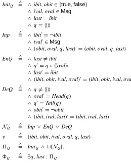
Q to the canonical form

given in Figure 3.5 _{Observe how each subaction}

Aof the original formula has a corresponding timed versionA

t_{. Action}

A

t _{is obtained by conjoining}

Awith the appropriate relations between the old and new values of the timers. If A has a lower-bound timer, thenA

t_{also has a conjunct asserting that it is not enabled when}

now is less than this timer. (The lower-bound timer tInpforInp does not affect the

enabling of other subactions because Inp is disjoint from all other subactions; a

similar remark applies to the lower-bound timertDeQ.) There is also a new action,

QTick, that advances now.

Formula5t

Qis the TLA specification of a program that satisfies each

maximum-delay constraint by preventingnow from advancing before the constraint has been

satisfied. Thus, the program “implements” timing constraints by stopping time, an apparent absurdity. However, the absurdity results from thinking of a TLA formula, or the abstract program that it represents, as aprescription of how something is

accomplished. A TLA formula is really adescription of what is supposed to happen.

Formula5t

Qsays only that an action occurs beforenow reaches a certain value. It

is just our familiarity with ordinary programs that makes us jump to the conclusion thatnow is being changed by the system.

3.2

Reasoning About Time

Formula5t

Qis a safety property; it is satisfied by a behavior in which no variables

change values. In particular, it allows behaviors in which time stops. We can rule

5_{Further simplification of this formula is possible, but it requires an invariant. In particular, the}

fourth conjunct ofDeQt_{can be replaced by T}0

InittQ 1

D ^ InitQ ^ now2R

^ tInp DnowCŽsnd

^ tDeQD TEnQDTDeQD 1

Inpt _D1 _{^ Inp} ^ tInp now

^ t0

Inp Dnow

0_CŽ

snd

^ T0

EnQ D if last06Dibit0then now0C1rcvelse1

^ .tDeQ;TDeQ/0 D if q D hh iithen.1;1/else.tDeQ;TDeQ/

^ now0_Dnow

En Qt _D1 _{^ En Q} ^ T0

EnQD 1

^ .tDeQ;TDeQ/0 D if q D hh iithen.nowCŽsnd; nowC1snd/

else .tDeQ;TDeQ/

^ .tInp;now/0D.tInp;now/

De Qt _D1 _{^ De Q} ^ tDeQnow

^ .tDeQ;TDeQ/0 D if q0D hh iithen.1;1/

else .nowCŽsnd; nowC1snd/

^ T0

EnQ D if last

0_Dibit0_{then1else T}

EnQ

^ .tInp;now/0D.tInp;now/

QTick D1 ^ now0₂._now;_min._T

DeQ;TEnQ/]

^ .v;tInp;tDeQ;TDeQ;TEnQ/0D.v;tInp;tDeQ;TDeQ;TEnQ/

vt D1 .v;now;tInp;tDeQ;TDeQ;TEnQ/

5t Q

1

D ^ Initt_Q

^ 2[Inp

t _{_ En Q}t _{_ De Q}t _{_ QTick]}

vt

Figure 3: The canonical form for5t

Q, where.r;s] denotes the set of reals u such

out such behaviors by conjoining to5t

Qthe liveness property

NZ D 81 t 2R :3.now>t/

which asserts thatnow gets arbitrarily large. However, when reasoning only about

real-time properties, this is not necessary. For example, suppose we want to show that our timed queue satisfies a real-time property expressed by formula9t_,

which is also a safety property. If5t

Qimplies9

t_{, then5}t

Q^NZ implies9 t

^NZ.

Conversely, we don’t expect conjoining a liveness property to add safety properties; if5t

Q^NZ implies9

t_{, then5}t

Qby itself should imply9

t_{—a point discussed in}

Section 3.3 below. Hence, there is no need to introduce the liveness propertyNZ.

A safety property we might want to prove for the timed queue is that it does not lose any inputs. To express this property, lethin be the history variable, determined

by Hin of (5), that records the sequence of input values; and lethout and Houtbe

the analogous history variable and property for the outputs. The assertion that the timed queue loses no inputs is expressed by

5t

Q^Hin^Hout ) 2.hout¼hinp/

whereÞ ¼ þ iffÞ is an initial prefix ofþ. This is a standard invariance property. The usual method for proving such properties leads to the following invariant

^ TQ ^ .tInp;now2R/ ^ .TEnQ;tDeQ;TDeQ2R[ f1g/

^ nowmin.TEnQ;TDeQ/

^ .lastDibit/ ) .TEnQD 1/ ^ .hinpDhoutŽq/

^ .last6Dibit/ ) .TEnQ<tInp/ ^ .hinpDhoutŽqŽ hhivalii/

^ .q D hh ii/ .TDeQD 1/

and to the necessary assumption1rcv < Žsnd. (Recall thatTQis the type-correctness

predicate (1) for5Q.)

PropertyNZ is needed to prove that real-time properties imply liveness properties.

The desired liveness property for the timed queue is that the sequence of input messages up to any point eventually appears as the sequence of output messages. It is expressed by

5t

Q^NZ ) 8¦ :2..hinpD¦/)3.houtD¦// This formula is proved by first showing

5t

and then using a standard liveness argument to prove

5t

Q^WFv.EnQ/^WFv.DeQ/ ) 8¦ :2..hinpD¦/)3.houtD¦// The proof that5t

Q^NZ implies WFv.EnQ/is by contradiction. AssumeEnQ is

forever enabled but never occurs. An invariance argument then shows that5t Q

implies thatTEnQforever equals its current value, preventingnow from advancing

past that value; and this contradictsNZ. The proof that5tQ^NZ implies WFv.DeQ/

is similar.

3.3

The NonZeno Condition

The timed queue specification5t

Q asserts that aDeQ action must occur between Žsnd and1snd seconds of when it becomes enabled. What if1snd < Žsnd? If an

input occurs, it eventually is put in the queue, enablingDeQ. At that point, the

value ofnow can never become more than1sndgreater than its current value, so

the program eventually reaches a “time-blocked state”. In a time-blocked state, only theQTick action can be enabled, and it cannot advance now past some fixed

time. In other words, eventually a state is reached in which every variable other thannow remains the same, and now either remains the same or keeps advancing

closer and closer to some upper bound.

We can attempt to correct such pathological specifications by requiring thatnow

increase without bound. This is easily done by conjoining the liveness propertyNZ

to the safety property5t

Q, but that doesn’t accomplish anything. Since5 t Q^NZ

rules out behaviors in whichnow is bounded, it allows only behaviors in which

there is no input, if1snd < Žsnd. Such a specification is no better than the original

specification5t

Q. The fact that the safety property allows the possibility of reaching

a time-blocked state indicates an error in the specification. One does not add timing constraints on output actions with the intention of forbidding input.

We call a safety propertyZeno if it allows the system to reach a state from which now must remain bounded. More precisely, a safety property5isnonZeno iff every

finite behavior satisfying5can be completed to an infinite behavior satisfying5 in whichnow increases without bound. In other words,5is nonZeno iff the pair

.5;NZ/is machine closed.6

Zeno specifications can be a source of incompleteness for proof methods. Only nonZeno behaviors are physically meaningful, so a real-time system with

specifi-6_{An arbitrary property5is nonZeno iff .}

cation5satisfies a property9if5^NZ)9. Most methods for proving safety properties use only safety properties as hypotheses, so they can prove5^NZ)9

for safety properties5and9only by proving5)9. NonZenoness of5means that5^NZ)9holds iff5)9does. However, if5is Zeno, then5^NZ)9

could hold even though5 ) 9 does not, and these methods will be unable to prove that the system with specification5satisfies9. NonZenoness is therefore required for completeness.

The following result can be used to ensure that a real-time specification written in terms of volatileŽ-timers is nonZeno.

Theorem 1 Letvbe the tuple of variables free in Init orN. The property ^Init^2[N]v^RTv

^ 8i 2 I : VTimer.ti;Ai; Ži; v/ ^MinTime.ti;Ai; v/

^ 8j 2 J : VTimer.Tj;Aj; 1j; v/ ^MaxTime.Tj/

is nonZeno if now does not appear inv, I and J are finite sets, and for all i 2 I and j 2 J:

1. hAjivis a subaction of Init^2[N]v whose free variables appear inv,

2. hAiiv andhAjivare disjoint for Init^2[N]vif i 6D j ,

3. Ži and1j are positive reals and, if i D j , thenŽi 1j,

4. the tiand Tjare distinct variables different from now and from the variables

inv.

We can apply the theorem to prove that the specification5t

Qis nonZeno ifŽsnd 1snd. The hypotheses of the theorem are checked as follows.

1. ActionshDeQi_vandhEnQi_vimplyNQ, so they are subactions of5Q.

2. The conjunction of any two of the actionshInpi_v,hDeQi_v, andhEnQi_vequals

false, so the actions are pairwise disjoint for5Q.7

3. The hypothesisŽsnd 1sndis used here.

7_{Actually, the type-correctness predicate T}

Q is needed to prove thathInpiv^ hDeQiv equals

4. Trivial.

The theorem is valid for persistent as well as volatile timers. Any combination ofVTimer and PTimer formulas may occur, except that a singleAk cannot have a persistent lower-bound timertk and a volatile upper-bound timer Tk. All of these

results are corollaries of the following theorem, which in turn is a consequence of Theorem 4 of Section 4.

Theorem 2 Let

ž 5be a safety property of the form Init^2[N]w,

ž ti and Tj be timers for5and letAk be an action, for all i 2 I , j 2 J, and

k2 I [ J, where I and J are sets, with J finite,

ž 5t _D1 5 _{^ RT} v ^

8i 2 I : MinTime.ti;Ai; v/ ^ 8j 2 J : MaxTime.Tj/

If 1. hAiiv and hAjiv are disjoint for5, for all i 2 I and j 2 J with

i6D j ,

now

2. (a) does not occur free inv,

(b) .now0_Dr/_^.v0_Dv/_{is a subaction of} 5_{, for all r2R,}

3. for all j 2 J: (a) hAjiv^.now

0_Dnow/_{is a subaction of}5_.

(b) 5 ) VTimer.Tj;Aj; 1j; v/, or

5 ) PTimer.Tj;Aj; 1j; v/, where1j 2.0;1/,

(c) 5t ₎

2.Enabled hAjiv D

Enabled .hAjiv ^ .now

0_Dnow///

(d) .v0 _Dv/ ₎ ._{Enabled h}

Ajiv D.Enabled hAjiv/ 0/

4. 5t ₎

2.tk Tk/, for all k 2 I \ J,

then.5t_{;NZ/is machine closed}

specifica-Theorem 2 can be further generalized in two ways. First, J can be infinite—if5t

implies that only a finite number of actionsAj with j 2 J are enabled before time

r , for any r 2 R. For example, by lettingAj be the action that sends message number j , we can apply the theorem to a program that sends messages number 1

throughn at time n, for every integer n. This program is nonZeno even though

the number of actions per second that it performs is unbounded. Second, we can extend the theorem to the more general class of timers obtained by letting the1j

be arbitrary real-valued state functions, rather than just constants—if all the1j are

bounded from below by a positive constant1.

Theorem 2 can be proved using Propositions 1 and 3 and ordinary TLA reasoning. By these propositions, it suffices to display a formulaL that is the conjunction of

fairness conditions on subactions of5t _{such that5}t_{^L implies NZ. A suitable L}

is WF_.now;v/.C/, whereCis an action that either (a) advancesnow by minj2J1j if allowed by the upper-bound timersTj, or else as far as they do allow, or (b) executes

an hAjiv action for which nowD Tj. The proof in the appendix of Theorem 4, which implies Theorem 2, generalizes this approach.

Theorem 2 does not cover all situations of interest. For example, one can require of our timed queue that the first value appear on the output line withinž seconds of when it is placed on the input line. This effectively places an upper bound on the sum of the times needed for performing theEnQ and DeQ actions; it cannot be

expressed withŽ-timers on individual actions. For these general timing constraints, nonZenoness must be proved for the individual specification. The proof uses the method described above for proving Theorem 2: we add to the timed program5t

a liveness property L that is the conjunction of any fairness properties we like,

including fairness of the action that advancesnow, and prove that5t_{^L implies}

NZ. NonZenoness then follows from Propositions 1 and 3.

There is another possible approach to proving nonZenoness. One can make granu-larity assumptions—lower bounds both on the amount by whichnow is incremented

and on the minimum delay for each action. Under these assumptions, nonZenoness is equivalent to the absence of deadlock, which can be proved by existing methods. Granularity assumptions are probably adequate—after all, what harm can come from pretending that nothing happens in less than 10 100_{nanoseconds? However,}

can be translated into a proof of nonZenoness using the method outlined above. So far, we have been discussing nonZenoness of the internal specification, where both the timers and the system’s internal variables are visible. Timers are defined by adding history-determined variables, so existentially quantifying over them preserves nonZenoness by Proposition 2. We expect most specifications to be fin [2, page 263], so nonZenoness will also be preserved by existentially quantifying over the system’s internal variables. This is the case for the timed queue.

3.4

An Example: Fischer’s Protocol

As another example of real-time closed systems, we treat a simplified version of a real-time mutual exclusion protocol proposed by Fischer [9], [12, page 2]. The example was suggested by Schneider [18]. The protocol consists of each process

i executing the following code, where angle brackets denote instantaneous atomic

actions:

a: awaithx D0i;

b: hx :Dii;

c: awaithx Dii;

cs: critical section

There is a maximum delay1b between the execution of the test in statementa and

the assignment in statementb, and a minimum delayŽcbetween the assignment in

statementb and the test in statement c. The problem is to prove that, with suitable

conditions on1b andŽc, this protocol guarantees mutual exclusion (at most one

process can enter its critical section).

As written, Fischer’s protocol permits only one process to enter its critical section one time. The protocol can be converted to an actual mutual exclusion algorithm. The correctness proof of the protocol is easily extended to a proof of such an algorithm.

The TLA specification of the protocol is given in Figure 4. The formula 5F

describing the untimed version is standard TLA. We assume a finite setProc of processes. Variablex represents the program variable x , and variable pc represents

the control state. The value ofpc will be an array indexed byProc, wherepc[i]

equals one of the strings “a”, “b”, “c”, “cs” when control in process i is at the

corresponding statement. The initial predicateInitFasserts thatpc[i] equals“a”for

each processi, so the processes start with control at statement a. No assumption

InitF D1 8i 2Proc:pc[i]D“a”

Go.i;u; v/ D1 ^ pc[i]Du

^ pc0_[i]

Dv

^ 8 j2 Proc:.j 6Di/ ) .pc0_{[j ]Dpc[ j ]/}

Ai

1

D Go.i;“a”;“b”/ ^ .x Dx0_D0/

Bi

1

D Go.i;“b”;“c”/ ^ .x0_Di/

Ci

1

D Go.i;“c”;“cs”/ ^ .x Dx0_Di/

NF

1

D 9i 2Proc:.Ai _ Bi _ Ci/

5F

1

D InitF ^ 2[NF].x;pc/

5t F

1

D ^ 5F ^ RT.x;pc/

^ 8i 2Proc :^ VTimer.Tb[i]; Bi; 1b; .x;pc// ^ MaxTime.Tb[i]/

^ 8i 2Proc :^ VTimer.tc[i]; Go.i;“c”;“cs”/; Žc; .x;pc// ^ MinTime.tc[i]; Ci; .x;pc//

8t F

1

D 9Tb;tc:5tF

Figure 4: The TLA specification of Fischer’s real-time mutual exclusion protocol.

a, b, and c. They are defined using the formula Go, where Go.i;u; v/ asserts that control in processi changes from u tov, while control remains unchanged in the other processes. ActionAi represents the execution of statementa by process

i; actionsBi andCi have the analogous interpretation. In this simple protocol, a process stops when it gets to its critical section, so there are no other actions. The program’s next-state actionNF is the disjunction of all these actions. Formula5F asserts that all processes start at statementa, and every step consists of executing

the next statement of some process.

ActionBiis enabled by the execution of actionAi. Therefore, the maximum delay of1bbetween the execution of statementsa and b can be expressed by an

upper-bound constraint on a volatile1b-timer for actionBi. The variableTbis an array of such timers, whereTb[i] is the timer for actionBi.

The constantŽcis the minimum delay between when control reaches statementc and

when that statement is executed. Therefore, we need an arraytc of lower-bound

statementc, so we want tc[i] to be aŽc-timer on an action that becomes enabled

when processi reaches statement c and is not executed untilCiis. A suitable choice for this action isGo.i;“c”;“cs”/.

Adding these timers and timing constraints to the untimed formula 5F yields

formula5t

Fof Figure 4, the specification of the real-time protocol with the timers

visible. The final specification, 8t

F, is obtained by quantifying over the timer

variablesTbandtc. SinceBj is a subaction of5F andpc[i]D“c”is disjoint from

Bj, for alli and j inProc, Theorem 2 implies that5

t

Fis nonZeno if1bis positive.

Proposition 2 can then be applied to prove that8t

F is nonZeno.

Mutual exclusion asserts that two processes cannot be in their critical sections at the same time. It is expressed by the predicate

Mutex D 81 i; j 2Proc:.pc[i]Dpc[ j ]D“cs”/).i D j/

The property to be proved is

Assump ^ 8t_F ) 2Mutex (8)

where Assump expresses the assumptions about the constantsProc, 1b, and Žc

needed for correctness. Since the timer variables do not occur inMutex or Assump,

(8) is equivalent to

Assump ^ 5t_F ) 2Mutex

The standard method for proving this kind of invariance property leads to the invariant

^ now2R

^ 8i2Proc:

^ Tb[i];tc[i] 2 R[ f1g ^ pc[i]2 f“a”;“b”;“c”;“cs”g ^ .pc[i]D“cs”/ ) ^ x Di

^ 8j 2Proc:pc[ j ]6D“b”

^ .pc[i]D“c”/ ) ^ x 6D0

^ 8 j 2Proc:.pc[ j ]D“b”/).tc[i] >Tb[j ]/ ^ .pc[i]D“b”/ ) .Tb[i]<nowCŽc/

^ now Tb[i]

and the assumption

4

Open Systems

A closed system is solipsistic. An open system interacts with an environment, where system steps are distinguished from environment steps. Sections 4.1 and 4.2 reformulate a number of concepts introduced in [1] that are needed for treating open systems in TLA. Some new results appear in Section 4.3. The following two sections explain how reasoning about open systems is reduced to reasoning about closed systems, and how open systems are composed.

4.1

Receptiveness and Realizability

To describe an open system in TLA, one defines an action¼ such that ¼ steps are attributed to the system and:¼ steps are attributed to the environment. A specification should constrain only system steps, not environment steps.

For safety properties, the concept of constraining is formalized as follows: if¼is an action and5a safety property, then5constrains at most¼iff, for any finite behaviors1; : : : ;sn and statesnC1, ifs1; : : :;sn satisfies 5and.sn;snC1/ is a:¼ step, then s1; : : : ;snC1 satisfies 5. The generalization to arbitrary properties of

constraining at most¼ is¼-receptiveness. Intuitively,5is¼-receptive iff every behavior in5can be achieved by an implementation that performs only¼steps— the environment being able to perform any:¼step. The concept of receptiveness is due to Dill [8]. The generalization to¼-receptiveness is developed in [1].8 _A

safety property is¼-receptive iff it constrains at most¼.

The generalization of machine closure to open systems ismachine realizability.

Intuitively, .5;L/ is ¼-machine realizable iff an implementation that performs only¼ steps can ensure that any finite behavior satisfying5is completed to an infinite behavior satisfying5^L. Formally,.5;L/ is defined to be¼-machine realizable iff.5;L/is machine closed and5^L is¼-receptive. For¼equal to

true, machine realizability reduces to machine closure.

8_{To translate from the semantic model of [1] into that of TLA, we let agents be pairs of states and}

identify an action¼with the set of all agents that are¼steps. A TLA behavior s1;s2; : : :corresponds

to the sequence s1

Þ2

!s2

Þ3

!s3

Þ4

!: : :, whereÞi equals.si 1;si/. With this translation, the

4.2

The

F

Operator

A common way of specifying an open system is in terms of assumptions and guarantees [10], requiring the system to guarantee a propertyM if its environment

satisfies an assumption E. An obvious formalization of such a specification is

the property E ) M. However, this property contains behaviors in which the

system violatesM and then the environment later violates E. Because the system

cannot predict what the environment will do, such behaviors cannot occur in any actual implementation. A behavior¦ generated by any implementation satisfies the additional property that if any finite prefix of¦ satisfies E, then it satisfies M.

We can therefore formalize the assumption/guarantee specification by the property

E F M, defined by: ¦ 2 E F M iff¦ 2 .E ) M/and, for every finite prefix

²of¦, if²satisfies E then² satisfiesM. If E and M are safety properties, then E F M is as well.

For safety properties, the operator Fis the implication operator of an intuitionistic logic [3]. Most valid propositional formulas without negation remain valid when

)is replaced by F, if all the formulas that appear on the left of a Fare safety properties. For example, the following formulas are valid if 8and5are safety properties.

8 F.5 F9/ .8^5/ F9

.8 F9/ ^ .5 F9/ .8_5/ F9

(9)

For any TLA formulas8and5, the property8 F 5is expressible as a TLA formula.

4.3

Proving Machine Realizability

Propositions 1–3, which concern machine closure, have generalizations for machine realizability. Proposition 1 is the special case of Proposition 4 in which8and¼ are identically true. Proposition 3 is similarly a special case of Proposition 5 if

.true;L2/is machine closed—that is, if L2is a liveness property. This is sufficient

for our purposes, sinceNZ is a liveness property. The generalization of Proposition 2

is omitted; it would be analogous to Proposition 10 of [1].

Proposition 4 is stated in terms of ¼-invariance, which generalizes the ordinary concept of invariance. A predicate P is a¼-invariant of a formula5iff, in any behavior satisfying5, no¼-step makes P false. This condition is expressed by

the TLA formula5)2[.¼^P/) P 0_]

Proposition 4 If 5and8are safety properties,5constrains at most¼, and L is the conjunction of a finite or countably infinite number of formulas of the form

WF_w.A/and/or SFw.A/, where, for each such formula,

1. hAiwis a subaction of 5^8,

2. 5^8)2[hAiw)¼]w,

3. if Aappears in a formula SFw.A/, then Enabled hAiw is a:¼-invariant

of 5^8,

then.8 F5; 8) L/is¼-machine realizable.

Proposition 5 If 8 and 5 are safety properties, .8 F 5;L1/ and .true;L2/ are ¼-machine realizable, and 8^5^ L1 implies L2, then .8 F 5;L2/ is ¼-machine realizable.

4.4

Reduction to Closed Systems

Consider a specificationE F M, where E and M are safety properties. We expect

the system’s requirement to restrict only system steps, meaning thatM constrains

at most¼. This implies that E F M also constrains at most¼. We also expect the environment assumptionE not to constrain system steps; formally, E does not constrain¼iff it constrains at most:¼and it is satisfied by every (finite behavior consisting only of an) initial state.9

SupposeE and M have the following form:

E D1 2[¼ _NE]v

M D1 Init ^ 2[:¼ _ NM]v

ThenE does not constrain¼andM constrains at most¼. If the system’s next-state actionNMimplies¼, and the environment’s next-state actionNE implies:¼, then a simple calculation shows that

E^M Init ^ 2[NE _NM]v (10)

Conjunction represents parallel composition, soE^M is the formula describing the

closed system consisting of the open system together with its environment. Observe

9_{The asymmetry between constrains at most and does not constrain arises because we assign the}

thatE^M has precisely the form we expect for a closed system comprising two

components with next-state actionsNE andNM.

We can make the inverse transformation from a closed system specification5to the corresponding assumption/guarantee specificationE F M such that5equals

E^M, where E does not constrain¼andM constrains at most¼. This is possible because any safety property5can be written as such a conjunction.

Implementation means implication. A system with guarantee M implements a

system with guaranteeM, under environment assumption E, iff Eb F M implies E F M. When E and M are safety properties, Eb F M implies E F M iffb E^M implies E^M. Thus, proving that one open system implements anotherb

is equivalent to proving the implementation relation for the corresponding closed systems. Implementation for open systems therefore reduces to implementation for closed systems.

4.5

Composition

The distinguishing feature of open systems is that they can be composed. The proof that the composition of two specifications implements a third specification is based on the following result, which is a reformulation of Theorem 2 of [1] for safety properties.

Theorem 3 If E, E1, E2,, M1, and M2 are safety properties and¼1 and¼2 are

actions such that

1. E1 does not constrain¼1 and E2does not constrain¼2,

2. M1 constrains at most¼1 and M2constrains at most¼2,

then the following proof rule is valid:

E^M1^M2 ) E1^E2

.E1 F M1/ ^ .E2 F M2/ ) .E F M1^M2/

This theorem is essentially the same as Theorem 1 of [3]; the proof is omitted.

5

Real-Time Open Systems

only decide how to separate timing properties into environment assumptions and system guarantees. An examination of a paradoxical example in Section 5.1 leads to the general form described in Section 5.2, where the concept of nonZenoness is generalized.

5.1

A Paradox

Consider the two componentsŠ1 and Š2 of Figure 5. Let the specification of

Š1 be Py F Px, which asserts that it writes a “good” sequence of outputs on x

if its environment writes a good sequence of inputs on y. Let Px F Py be the

specification ofŠ2, soŠ2writes a good sequence of outputs ony if its environment

writes a good sequence of inputs onx . If Px and Pyare safety properties, then it

appears that we should be able to apply Theorem 3, our composition principle, to deduce that the composite systemŠ12satisfies Px^Py, producing good sequences

of values onx and y. (We can define¼1and¼2so that writing onx is a¼1 action and writing ony is a¼2action.)

Now, suppose Px and Py both assert that the value 0 is written by noon. These

can be regarded as safety properties, since they assert that an undesirable event never occurs—namely, noon passing without a 0 having been written. Hence, the composition principle apparently asserts thatŠ12sends 0’s along bothx and y by

noon. However, the specifications ofŠ1andŠ2are satisfied by systems that wait for a 0 to be input, whereupon they immediately output a 0. The composition of those two systems does nothing.

This paradox depends on the ability of a system to respond instantaneously to an input. It is tempting to rule out such systems—perhaps even to outlaw specifications like these. We show that this Draconian measure is unnecessary. Indeed, if the specification ofŠ2is strengthened to assert that a 0 must unconditionally be written on y by noon, then there is no paradox, and the composition does guarantee that a

0 is written on bothx and y by noon. All paradoxes disappear when one carefully

examines how the specifications must be written.

To resolve the paradox, we examine more closely the specificationsS1 andS2 of Š1andŠ2. For simplicity, let the only possible output actions be the setting ofx

and y to 0. The untimed version of S1 then asserts that, if the environment does