Electrocatalysis in Solid Acid Fuel Cell Electrodes

Electrocatalysis in Solid

Acid Fuel Cell Electrodes

Thesis by

Vanessa Evoen

In Partial Fulfillment of the Requirements for the Degree of

Doctor of Philosophy

CALIFORNIA INSTITUTE OF TECHNOLOGY Pasadena, California

2016

 2016

Vanessa Evoen

This work would not have been possible without financial support from the National Science Foundation (NSF), Gordon and Betty Moore foundation (via the Caltech Center for the Science and Engineering of Materials), and the Advanced Research Projects Agency-Energy (ARPA-E). In addition, I am thankful to the NSF Graduate Research Fellowship Program (GRFP) for three years of support.

I am forever grateful to my thesis advisor Professor Sossina Haile, who has been an inimitable advisor. She is great at identifying the best experiment to do next, which makes for exciting scientific discoveries. I am grateful for all of her personal and professional insight, and for her guidance through my graduate school career. She is a great role model for women in science, and I am thankful for the opportunity to work with her. I am also grateful to have met her wonderful kids Alem and Hanu, who have been a joy to get to know.

I would like to acknowledge Professor Robert Hicks for being a great mentor while I was an undergraduate at UCLA. He encouraged me to pursue a PhD, and wrote me great letters of recommendation for graduate school and graduate fellowships. His infinite enthusiasm for science was encouraging and inspiring. I am grateful for all his support, and I am thankful that he encouraged me at a very early stage to tackle graduate-level scientific research.

I am thankful to Professor Sarah Tolbert at UCLA and Professor Paula Hammond at MIT for giving me the opportunity as an undergraduate, to work with graduate students in their research groups. These opportunities exposed to me to a variety of research fields and expanded my skill set in the laboratory. Most importantly, these experiences shaped a solid foundation for my graduate research career. Finally, I am grateful for their recommendation letters for graduate school applications and graduate fellowships.

access to his group’s COMSOL license. Finally, I would like to thank Professor Rick Flagan for serving on my candidacy committee. His insight into my PhD work was very helpful in shaping the direction of my research.

There are many individuals to whom I owe my gratitude for various contributions to my progress at Caltech. I am grateful to Calum Chisholm for fruitful discussions about solid acids and for granting access to test stations at SAFCell. I am grateful to Mandy Abbott and Fernando Campos for providing samples for research purposes and for answering questions regarding solid acid fuel cell (SAFC) test station construction. I would like to thank the supportive staff at Caltech, Dr. Felicia Hunt, Natalie Gilmore and Teresita Legaspi for the countless work they do to support students every day.

I have worked with a lot of researchers at Caltech that I have learned a great deal from. I am grateful to Aron Varga for teaching me how to electrospray. I am thankful to Moritz Pfohl for showing me how to use the chemical vapor deposition (CVD) setup. His recommendations for improving the setup were helpful in generating reproducible results. I am thankful to Jaemin Kim for teaching me how to take impedance measurements. I would like to acknowledge Hadi Tavassol, who helped with polarization curve measurements and stability studies. He was an encouraging partner on the solid acid team. I would also like to thank Tim Davenport who taught me how to do mass spectrometry measurements and thermal stability studies. Tim is one of the most helpful people I have worked with at Caltech. I would like to acknowledge Nick Brunelli who helped with synthesizing nickel nanoparticles used for all of the in-house grown carbon nanotubes studied in this work. Finally, I would like to thank Mike Ignatowich, whose thermochemical test station I used for reactivity studies at Northwestern university.

great collaborator and friend in the solid acid team. I would like to acknowledge recent additions to the solid acid team, Sheel Sanghvi and Shobhit Pandey. It has been great to work with them, as they effectively start their graduate research. I would like to acknowledge friends I have made in the Haile/Snyder group like Chirranjeevi Balaji Gopal (BG), Moureen Kemei, Philipp Simons, Yinglu Tang, Carolyn Richmonds, Jenny Schmidt, Tristan Day, and Hyunsik Kim. At any point, I could rely on any of them for support and encouragement on the third floor of Steele Labs, and I am grateful.

I forged lifelong bonds with people I met during my first year in chemical engineering at Caltech. I would like to thank Marilena Dimotsantou for being a great friend and roommate. We had so much fun together and saw each other through some tough times. I would like to thank Charlie Slominski, Ricardo Bermejo-Deval and Kate Fountaine for being great friends and roommates. Finally, Kat Fang for being the best study partner. I was fortunate to meet other amazing friends in other departments like Eyrun Eyjolfsdottir, Steve Demers, Ryan Henning, Jean Pierre-Voropaieff, Georgia Papadakis, and Marius Lemm. I had so much fun getting to know you all.

I have had many supportive friends outside of graduate school who have made this journey so much better. I would like to thank Jennifer Guerrerro and Basak Kilic, who have been my best friends since my undergraduate days at UCLA. I would like to acknowledge Amaka Liz James for being a great friend and always providing a necessary break from academia from time to time. Thank you to all my supportive friends over the years like Kehinde and Taiwo Osuntola and Eleanor Okubor.

I would like to acknowledge Joanna and Don Gwinn, who opened up their home to me in Evanston, Illinois. You made the transition from Caltech to Northwestern so much easier when I moved in with you. Thank you for giving me a home away from home.

Fuel cells are appealing alternatives to combustion engines for efficient conversion of chemical energy to electrical energy, with the potential to meet substantial energy demands with a small carbon footprint. Intermediate temperature fuel cells (200-300oC) combine the kinetic benefits and fuel flexibility of higher operating temperatures along with the flexibility in material choices that lower operating temperatures allow. Solid acid fuel cells (SAFCs) offer the unique benefit amongst intermediate temperature fuel cells of a truly solid electrolyte, specifically, CsH2PO4, which in turn, provides significant system

simplifications relative to phosphoric acid or alkaline fuel cells9, 10 However, the power output of even the most advanced SAFCs has not yet reached levels typical of conventional polymer electrolyte or solid oxide fuel cells. This is largely due to poor activity of the cathodes. That is, while it has been possible to limit electrolyte voltage losses in SAFCs through fabrication of thin-membrane fuel cells (with electrolyte thicknesses of 25–50 μm), it has not been possible to attain high activity cathodes or to limit Pt loadings to competitive levels.1 In this thesis, the efficacy of non-precious metal catalysts in the solid acid electrochemical system is evaluated. In addition, an attractive synthesis route (specifically, the electrospray method) to fabricating high surface area electrodes with high catalyst utilization is presented.

spectroscopy and fuel cell measurements, were significantly enhanced by chemical functionalization with oxygen containing functional groups. Area normalized impedance responses as low as 7 Ω cm2 _{were measured on symmetric MWCNT/ CsH}

2PO4 cells.

However, it was discovered that these reactive MWCNTs also catalyze and are slightly consumed by steam reforming. Moreover, the orders of magnitude improvement with functionalization measured in impedance measurements is not replicated in fuel cell power output as a result of a decrease in open circuit voltage relative to standard cells. It is proposed that the loss in voltage results from hydrogen production at the cathode via the steam reforming reaction, although formation of hydrogen peroxide rather than water as the oxygen reduction product cannot be ruled out. This work has a significant contribution to catalysis, it demonstrates how carbon nanostructures can be designed by synthesis routes and chemical functionalization processes, to create active precious-metal-free ORR catalysts. It is also important that we have demonstrated potential ORR catalysts in acidic media. These catalysts have potential applications in phosphoric acid fuel cells and PEMFCs.

In addition to the study of carbon nanostructures, oxides were evaluated as potential ORR catalysts. Specifically, TiOx nanoparticles were studied. Analysis shows that the

activity is controlled by the oxidation state of Ti. The active site seems to be on or near slightly reduced Ti sites. In this study we have outlined synthesis routes to tune the oxidation state of Ti and enhance ORR activity in the solid acid fuel cell.

ACKNOWLEDGEMENTS ... iii

ABSTRACT... vi

TABLE OF CONTENTS ... viii

LIST OF FIGURES ... x

NOMENCLATURE ... xvii

CHAPTER 1. Introduction ... 1

1.1 Overview... 1

1.2 Fuel cells ... 1

1.3 Solid Acid Fuel cells ... 5

1.3.1 Solid Acid compounds ... 5

1.3.2 Solid acid fuel cells (SAFCs); basics, challenges and current status ... 9

1.4 Objectives of this thesis ... 15

CHAPTER 2. Experimental methods ... 16

2.1 Characterization techniques ... 16

2.1.1 Electrochemical characterization (in situ) ... 16

2.1.2 Ex situ characterization ... 26

2.2 Synthesis methods ... 29

2.2.1 Electrospray deposition ... 29

CHAPTER 3. Electrochemistry as a tool for evaluating the reactivity of carbon ... 35

Section 3.1 Accessing the efficacy of MWCNTs in SAFCs ... ...35

3.1.1. Introduction ... 35

3.1.2. Experimental ... 37

3.1.3. Results and discussion ... 39

3.1.4. Conclusion ... 54

Section 3.1. Supplemental material... 56

Section 3.2. Parametric Study on MWCNT oxygen reduction reaction activity (ORR) ... 62

3.2.1. Overview ... 62

3.2.2. Results and discussion ... 66

3.2.3. Conclusion ... 71

CHAPTER 4.Tuning the reactivity of carbon nanostructures by growth parameters ... 72

4.1. Abstract ... 72

4.4. Results and discussion ... 79

4.5. Conclusion ... 97

4.6. Acknowledgement ... 98

CHAPTER 5.Oxygen reduction by TiOx overlayers ... 99

5.1. Introduction ... 99

5.2. Experimental ... 99

5.3. Results and discussion ... 100

5.4. Conclusion ... 111

CHAPTER 6. Electrospray of nano-sized CsH2PO4 for SAFC electrodes ... 112

Section 6.1. In situ characterization of electrosprayed CsH2PO4 solid acid nanoparticles ... 112

6.1.1. Abstract ... 112

6.1.2. Introduction ... 112

6.1.3. Electrospray background ... 114

6.1.4. Experimental procedures ... 117

6.1.5. Results ... 122

6.1.6. Discussion ... 130

6.1.7. Conclusions ... 133

Section 6.1. Supplementary material ... 135

Solvent evaporation of a single µm sized droplet ... 135

Section 6.2. Electrospray throughput ... 140

6.2.1. Experimental details... 141

6.2.2. Results and discussion ... 145

6.2.3. Conclusion ... 160

IMPACTS AND INSIGHTS ... 162

Chapter 1

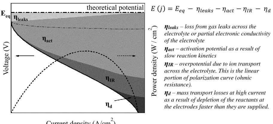
Figure 1.1. Schematic of a fuel cell polarization curve, with contributions of various overpotentials

indicated by the shaded regions, and explained on the right. The power density (dotted line) is the product of the cell voltage and current density ... 3

Figure 1.2. Schematic of a typical porous composite electrode showing a proton conducting electrolyte,

electron conducting catalyst, and gas phase species (O2), that comprise a triple phase boundary

(TBP) point. ... 4

Figure 1.3. Arrhenius plot of proton conductivity, σH, of a few solid acid compounds that exhibit a

super-protonic phase transition. 203 _{... 6}

Figure 1.4. Super-protonic phase transition in CsH2PO4. (a) Arrhenius plot of proton conductivity (σ), in

humidified N2. (b) Unit cells of monoclinic and cubic phases.2, 3 ... 7

Figure 1.5. Phase stability regions of CsH2PO4 adapted from Taninouchi et al.5 and Chisholm et al.9 ... 8

Figure 1.6. Schematic of a fuel cell depicting the anode and cathode half reactions.4 _{... 9}

Figure 1.7. (a) IR corrected solid acid fuel cell polarization plot showing small ohmic losses in comparison

to other sources of overpotential loss.4 _{(b) Cathode and anode contributions to the overpotential of a}

SAFC.29 _{... 10}

Figure 1.8. Comparison of IR-free polarization curves of SAFCs incorporating different sized CsH2PO4 in

the cathode. Scanning electron micrographs are shown below.1 _{... 11}

Figure 1.9. (a) SEM micrographs of composite electrode nanostructures comprising CsH2PO4, Pt-black

and poly-vinylpyrrolidone (PVP). (b) Impedance spectra of representative CsH2PO4 +

Pt|CsH2PO4|CsH2PO4 + Pt symmetric, electrochemical cells with electrosprayed electrodes on

carbon and a Pt loading of 0.3 ± 0.2 mg/cm2_{; data collected under humidified hydrogen with pH} 2O =

0.4 atm at 240 0_C.7 _{... 12}

Figure 1.10. Impedance spectra of four CsH2PO4 + Pt +PVP composite electrodes electrosprayed onto

CNTs, and one without CNTs but otherwise identical.6 _{... 13}

Figure 1.11. (a) Synthetic approach for Pt decorated CNTs. (b) Electrospray deposition strategy of Pt-CNT

+ CsH2PO4 composites. (c) Symmetric cell impedance measurements of 30 wt % Pt-CNT based

electrodes. Measurements performed in humidified H2 (pH2O = 0.4 atm) and Pt loading is 5.1 E-3

mg/cm2_{. Inset is equivalent circuit used for fitting.}8 _{... 13}

Chapter 2

Figure 2.1. (a) The j-η representation of a hypothetical electrochemical reaction. The Tafel approximation

deviates from Butler-Volmer kinetics at low overpotentials.10 _{(b) Effect of overpotential on fuel cell}

performance. ... 18

Figure 2.2. (a) Application of a small signal perturbation confines the impedance measurement to a

pseudo-linear portion of a fuel cell’s I-V curve (b) A sinusoidal voltage perturbation and resulting current response with a phase shift (θ) ... 19

Figure 2.3. (a) Nyquist plot of a hypothetical fuel cell. Regions marked correspond to ohmic, anode

activation and cathode activation losses, respectively. (b) Schematic of a fuel cell with cathode and anode half reactions... 20

Figure 2.4. (a) An illustration of the movement of a proton under electric field perturbation at varying

anode cell. ... 22

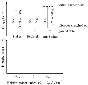
Figure 2.6. (a) Schematic of Stokes, Rayleigh and anti-Stokes scattering. (b) Scattered Raman spectrum

intensities plotted against relative wave numbers. ... 27

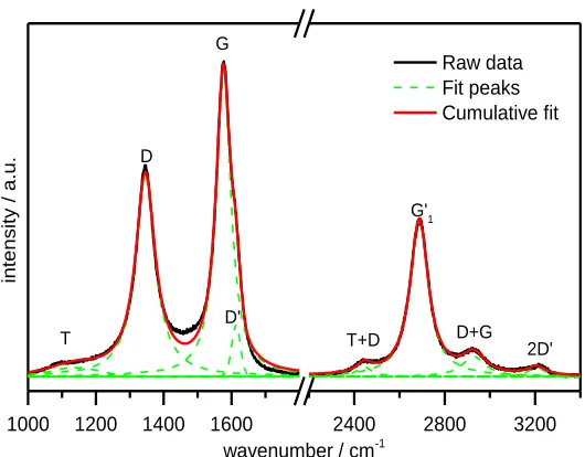
Figure 2.7. First and second-order Raman spectra of a carbon nanotube material. Background corrected

spectrum is shown in black, fitted peaks in green dashed lines and cumulative fit peak is shown in red. ... 28

Figure 2.8. A schematic of electrospray ionization, the effluent leaves the Taylor cone as charged droplets

that undergo columbic explosions at the Rayleigh limit. ... 30

Figure 2.9. Four types of film morphologies obtained by electrospray. I, dense film; II, dense film with

incorporated particles; III, porous top layer with dense bottom layer; IV, fractal-like porous

structure, according to Chen et al.60 _{... 31}

Figure 2.10. Initial droplet velocity of the emitted droplet of varying solid acid concentration. ... 33

Chapter 3

Figure 3.1. (a) Fourier-Transform infrared (FTIR) spectra of hollow CNTs, CNT-NH2 and CNT-COOH.

Dashed lines identify peaks corresponding to labelled functional groups. (b) First order Raman spectra of the CNTs, CNT-NH2 and CNT-COOH. The dashed lines specify the peak position of the D

band, G band and D’ band. The defect density characterized as the ratio of the D band intensity to the G band intensity is shown inset. ... 41

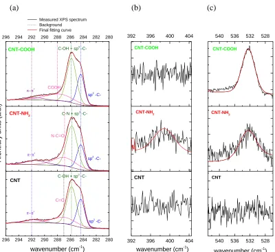
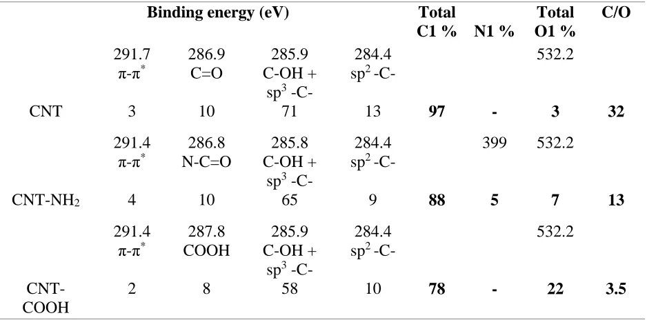
Figure 3.2. Deconvolution of the XPS (a) C1s, the (b) N1s and (c) O1s spectra of the CNTs, CNT-NH2 and

CNT-COOH. ... 42

Figure 3.3. TGA profiles for hollow MWCNTs, MWCNT-NH2 and MWCNT-COOH measured under

flowing air at a heating rate of 2 0_{C/min. ... 44}

Figure 3.4. (a) Ion current ratio of H2 to H2O for 400 mg of hollow CNT, hollow CNT-NH2 and hollow

CNT-COOH at pH2O = 0.2 atm and 8000C. (b) Ion current ratio of H2 to H2O for 400 mg of hollow

CNT and hollow CNT-COOH with varying pH2O. ... 45

Figure 3.5. Arrhenius plot of H2 ion current versus inverse temperature of the cool down and heat up

between 8000_{C to 600}0_{C of 200 mg of CNT-COOH (ramp rate is 100} 0_{C/ hour). ... 46}

Figure 3.6. a) SEM images of Hollow MWCNTs 15 ± 5 nm in outer diameter, 5-20 µm in length.

Cross-sectional SEM images of symmetric pellets with 600mg of CsH2PO4 electrolyte sandwiched between

50mg 1:1 MWCNT: CsH2PO4 composite electrodes of b) Hollow MWCNTS, c) Hollow

MWCNTs-NH2, d) Hollow MWCNTs-COOH. ... 47

Figure 3.7. Measurements performed at 250 °C under humidified O2 and H2 gases (pH2O = 0.4 atm) at a

flow rate of 40 sccm. (a) Four H2/O2 polarization curves (IR corrected) measured consecutively

between 0.0V and 0.95 V on 50mg 1:1 CNT: CsH2PO4 composite cathode and 25 mg 1:3 Pt/C :

CsH2PO4 anode. Fuel cell polarization curve recorded at 2.5mv/s for CNTs, CNT-NH2 and

CNT-COOH electrodes. Inset is the open circuit potential (OCP). (b) Impedance measurements on the fuel cell, at equilibrium in the frequency range of 10 mHz to 0.2 MHz. Inset is the impedance model fit which is a finite length Warburg element (Ws) and a resistor in series with a resistor (R) and constant

phase element (CPE) in parallel. Impedance measurements were taken on the cell before the polarization curves were measured. (c) Open circuit potential versus area normalized impedance from impedance curve fits. (d) Summary of impedance curve fitting. ... 48

Figure 3.8. Measurements performed at 250°C under humidified oxygen (pH2O = 0.4atm) flowing at 40

sccm. (a) Comparison of Symmetric cell impedance measurements of 50mg 1:1 CNT: CsH2PO4

composite electrodes of MWCNTs, MWCNTs-NH2 and MWCNTs-COOH in humidified O2 in a

Nyquist representation (ω=10 KHz – 5 mHz). Inset is the impedance model fit which is a finite length Warburg element (Ws) and a resistor in series with a resistor (R) and constant phase element (CPE)

and the total resistance (RTOT). ... 49

Figure 3.9. Long term degradation behavior of MWCNTs. (a) Symmetric impedance measurements in

humidified O2 (pH2O = 0.4atm). Rrel is the electrochemical resistance of 50 mg 1:1 CNT : CsH2PO4

composite electrodes at time (t) divided by electrochemical resistance measured 10 min after O2 is

flowed to the cell.Inset is an SEM image of MWCNT over-grown carbon paper used as a current collector to improve electrode stability. (b) Comparison of symmetric cell impedance measurements of 50mg 1:1 CNT: CsH2PO4 composite electrodes of hollow MWCNTs, hollow MWCNT after

12-hour treatment in air and hollow MWCNT after 12-12-hour treatment in humidified O2. Measurements

performed at 2500_{C under humidified O}

2 gas flowing at 40 sccm (ω=10 KHz – 5 mHz). ... 51

Figure 3.10. (a) Forward and reverse hydrogen oxidation and oxygen reduction half reactions at the anode

and cathode, respectively, in fuel cell configuration. (b) The oxygen reduction reaction and the steam reforming reaction at the electrodes in symmetric cell configuration. The proposed carbon corrosion reaction is highlighted in blue and the oxygen reduction reaction is highlighted in red. ... 53

Figure 3.11. (a) First scan of the I-V curve measured in Figure 3.6. Inset shows that the cathodic branch of

the I-V curve has a higher OCP than the anodic branch of the fuel cell I-V curve. (b) The average OCP value (where the I-V curve crosses the zero current density line) for the cathodic and anodic branch of the I-V curve versus the average slope at zero current ... 54

Figure 3.S.1. Comparison of electrode responses for 50 mg 1:1 CNT : CsH2PO4 composite electrodes in

humidified (pH2O = 0.4atm) under Ar at the cathode and H2 at the anode. ... 56

Figure 3.S.2. (a) Comparison of electrode responses for 50 mg 1:1 CNT : CsH2PO4 composite electrodes

in humidified (pH2O = 0.4atm) under symmetric argon. (b) Log-log plot of |z(ω)2|versus 1/ω, where

the offset is (R0)2/τ. ... 57

Figure 3.S.3. Symmetric impedance measurements in humidified O2 (pH2O = 0.4atm). Rrel is the

electrochemical resistance of 25 mg 1:1 CNT : CsH2PO4 composite electrodes at time (t) divided by

electrochemical resistance measured 10 min after O2 is flowed to the cell ... 57

Figure 3.S.4. (a) Symmetric cell AC impedance measurements of 1:1 hollow CNT-COOH: CsH2PO4

composite electrodes in humidified O2 (pH2O=0.4 atm). Electrode loading was 25mg, 50mg and

100mg, respectively. (b) Plot of average area specific resistance (ASR) from fitting impedance data versus mass of 1:1 hollow CNT-COOH : CsH2PO4 composite electrodes. The error bars correspond

to the standard deviation in ASR over the number of samples measured (in set). ... 58

Figure 3.S.5. (a) Comparison of symmetric cell impedance measurements of 50mg 1:1 CNT: CsHSO4

composite electrodes of Hollow MWCNTs-COOH. Measurements performed at 1650_{C in symmetric}

60 sccm O2 and varying pH2O. (b) Electrode resistance from impedance fitting with varying pH2O.

(c) Electrode impedance from R (ω=0.005 Hz) - R (ω=1000 Hz) with varying pH2O. ... 59

Figure 3.S.6. RDE polarization curves for Hollow MWCNTs and Hollow MWCNTs-COOH. 5 mg of

Hollow MWCNT and 10 mg of hollow MWCNT-COOH were suspended respectively, in 450µL of ethanol, 450µL of isopropanol and 100 µL of Nafion. 5 µl of the resulting carbon nanotube ink was deposited on the glassy carbon electrode. In a) polarization curves in acidic media are shown for 0.1 M HClO4, 0.1 M phosphate buffer, and 0.1 M acetate buffer. (b)Ppolarization curves in 0.1 M KOH

are shown for MWCNTs in comparison with Pt/C. In c) the onset voltage at -1mA/cm2 _{is summarized}

for all MWCNTs in acidic and basic media. ... 60

Figure 3.S.7. Average area specific resistance (ASR) or area normalized impedance (from symmetric cell

AC impedance measurements in humidified O2) versus the mass loading of the CNT electrodes. This

shows that the 1:1 mass ratio loading had the highest ORR activity, hence was used for all

measurements. ... 61

length is 5– 10 µm) and bamboo MWCNTs (OD is 30 ± 5 nm and length is1-5 µm). ... 63

Figure 3.2.3. Measurements performed at 2500_{C under humidified oxygen (pH}

2O = 0.4atm) flowing at 40

sccm. Comparison of symmetric cell impedance measurements of 50mg 1:1 CNT: CsH2PO4

composite electrodes in a Nyquist representation (ω=10 KHz – 5 mHz). ... 63

Figure 3.2.4. a) First order Raman spectra of hollow and bamboo MWCNTs. The dashed lines specify the

peak position of the D band, G band and D’ band. The defect density characterized as the ratio of the D band intensity to the G band intensity is shown inset. b) Fourier-transform infrared (FTIR) spectra of hollow and bamboo MWCNTs. Dashed lines identify peaks corresponding to labelled functional groups. ... 64

Figure 3.2.5. Plot of average area specific resistance (ASR) from fitting impedance data versus type of

CNT used in 50 mg 1:1 mass ratio CNT : CsH2PO4 composite electrodes. The error bars correspond

to the standard deviation in ASR. ... 65

Figure 3.2.6. Area normalized impedance from impedance measurements versus outer diameter (OD) and

length (L) of hollow and bamboo variation MWCNTs. ... 66

Figure 3.2.7. ID/IG (from Raman measurements) for all varying hollow and bamboo MWCNTs

characterized, versus area normalized impedance values (from symmetric cell AC impedance measurements in humidified O2). Brackets indicate that the shorter MWCNTs of both variations have

higher measured ID/IG. ... 67

Figure 3.2.8. BET surface area for all varying hollow and bamboo MWCNTs characterized, versus area

normalized impedance values (from symmetric cell AC impedance measurements in humidified O2).

... 68

Figure 3.2.9. Area normalized impedance from symmetric AC impedance measurements in humidified O2

versus the relative concentration of the carbonyl (C=O) functional group in the hollow/bamboo MWCNT. ... 70

Chapter 4

Figure 4.1. (a) Schematic diagram of tip growth model at different time steps. (b) The MWCNT in the tip

growth scheme depicting the (i) catalyst particle, (ii) embryo and (iii) full grown MWCNT

(Reproduced from Hembram et al.).81 _{... 74}

Figure 4.2. SEM micrographs of MWCNTs grown with 80 nm Ni seed catalyst and growth temperature

800 °C in; (a) 𝑃𝐶2𝐻2 = 0.016 𝑎𝑡𝑚: 16 sccm C2H2, 750 sccm Ar, 250 sccm H2 and (b) 𝑃𝐶2𝐻2 = 0.060 𝑎𝑡𝑚: 16 sccm C2H2, 250 sccm H2. Inset is higher magnification. ... 79

Figure 4.3. STEM images of MWCNTs grown with 80 nm Ni seed catalyst and growth temperature 800

°C in (a) 𝑃𝐶2𝐻2 = 0.016 𝑎𝑡𝑚. Dashed lines show the ‘bamboo’ like structure of the MWCNTs. (b)

𝑃𝐶2𝐻2 = 0.060 𝑎𝑡𝑚. Dark spots are amorphous carbon deposits... 80

Figure 4.4. First order Raman spectra measured for MWCNTs grown with 𝑃𝐶2𝐻2 = 0.016 𝑎𝑡𝑚 (top) and

𝑃𝐶2𝐻2 = 0.060 𝑎𝑡𝑚 (bottom). (a) 80 nm Ni seed catalyst. (b) 40 nm Ni seed catalyst. The dashed lines indicate the peak position of the D band, G band and D’ band. The defect density characterized as the ratio of the D band intensity to the G band intensity is shown inset. In all cases, the growth temperature is 800 °C. ... 82

Figure 4.5. a) Comparison of symmetric cell impedance measurements of 50mg 1:1 CNT: CsH2PO4

composite electrodes (varied parameters shown inset and growth temperature is 800 °C) in a Nyquist representation (ω=10 KHz – 5 mHz). Measurements collected at 2500_{C under humidified O}

2 (pH2O

= 0.4atm) flowing at 40 sccm. (b) Area normalized impedance versus ID/IG ratios from Raman

characterization. ... 83

Figure 4.8. Deconvolution of the XPS C1s peak for MWCNTs grown at 𝑃𝐶2𝐻2 = 0.060 𝑎𝑡𝑚, ... 85

Figure 4.9. First order Raman spectra measured for MWCNTs grown with 𝑃𝐶2𝐻2 = 0.60 𝑎𝑡𝑚 and 80 nm Ni seed, at 800 °C; (a) HNO3 treated and (b) untreated MWCNTs. The dashed lines specify the

peak position of the D band, G band and D’ band. ID/IG and ID’/IG is shown inset. ... 87

Figure 4.10. Comparison of symmetric cell impedance measurements of 50mg 1:1 MWCNT: CsH2PO4

composite electrodes in a Nyquist representation for untreated and HNO3 treated MWCNTs.

Measurements were collected at 2500_{C under humidified O}

2 (pH2O = 0.4atm) flowing at 40 sccm in

the 5mHz to 10KHz frequency range. Inset is higher magnification. MWCNTs grown in 𝑃𝐶2𝐻2 = 0.060 𝑎𝑡𝑚, growth temperature = 800 °C, and 80 nm Ni seed catalyst. ... 88

Figure 4. 11. SEM images of MWCNTs grown in 𝑃𝐶2𝐻2 = 0.060 atm with 80 nm Ni particles at 600 °C, 650 °C, 700 °C, and 800 °C. Inset is higher magnification ... 89

Figure 4.12. First order Raman spectra measured for HNO3 -treated MWCNTs grown with 𝑃𝐶2𝐻2 = 0.060 𝑎𝑡𝑚 and 80 nm Ni seed catalyst; (a) fit with D band, G band and D’ band (b) D band, G band D’ band, and T2 band. Growth temperature is inset. ... 90

Figure 4.13. FWHM of the ‘D’ peak in Raman measurements versus growth temperature. ... 91 Figure 4.14. Deconvolution of the XPS C1s peak for MWCNTs grown at 𝑃𝐶2𝐻2 = 0.060 𝑎𝑡𝑚 with 80 nm Ni seed catalyst at a growth temperature of (a) 600 °C, (b) 650 °C, (c) 700 °C, and (d) 800 °C ... 92

Figure 4.15. Deconvolution of the XPS C1s peak for HNO3 treated MWCNTs grown at 𝑃𝐶2𝐻2 = 0.060 𝑎𝑡𝑚 with 80 nm Ni seed catalyst at a growth temperature of (a) 600 °C, (b) 650 °C, (c) 700 °C, and (d) 800 °C. ... 93

Figure 4.16. Deconvolution of the XPS N1s peak for MWCNTs grown at 𝑃𝐶2𝐻2 = 0.060 𝑎𝑡𝑚 with 80 nm Ni seed catalyst at a growth temperature of (a) 600 °C, (b) 650 °C, (c) 700 °C, and (d) 800 °C (CPS refers to counts per second). ... 94

Figure 4.17. Comparison of symmetric cell impedance measurements of 50mg 1:1 MWCNT: CsH2PO4

composite electrodes in a Nyquist representation for HNO3 treated MWCNTs. Measurements were

collected at 2500_{C under humidified O}

2 (pH2O = 0.4atm) flowing at 40 sccm in the 5mHz to 10KHz

frequency range. MWCNTs grown in 𝑃𝐶2𝐻2 = 0.060 𝑎𝑡𝑚 with 80 nm Ni seed catalyst. The growth temperature is inset. ... 96

Figure 4.18. Average area normalized impedance values versus the % Oxygen from XPS analysis of HNO3

treated MWCNTs grown with 𝑃𝐶2𝐻2 = 0.16 𝑎𝑡𝑚 and 80 nm Ni seed catalyst ... 97

Chapter 5

Figure 5.1. (a) Polarization behavior and (b) phase fraction of the as-received TiO2 micropowders of rutile

(R) and anatase (A). ... 102

Figure 5.2. (a) Phase fraction of rutile and anatase TiO2 in the oxide layers grown on Ti metal powders.

(b) Polarization response of different Ti-based cathodes, and comparison with a Pt on carbon black cathode. R and A represents as received rutile and anatase micro-powders. Polarization curves represented are from Titanium micro-powders treated at shown temperatures for 30 min under 0.7% O2 (Ar balance). (c) Cell voltage of the titania cathodes shown in part b at 5 mA cm-2 of current. .. 104

Figure 5.3. Cell voltage with cathodes made from titanium micropowders annealed at 600 °C, under 0.7%

O2 (balance Ar) for different growth times. Voltage is compared at 5 mA cm-2 of current. Gray bars

represent the cathodes following five electrochemical cycles between 0.95 V and 0V at a scan rate of 2.5 mV s-1_{. ... 105}

Figure 5.4. Samples prepared from titanium metal micropowder (a) before annealing; and after annealing

at 600 °C in 0.7% O2 (balance Ar) for (b) 15 min, (c) 30 min and (d) 60 min. ... 106

Figure 5.5. Rutile and anatase phase fractions of the powder samples following annealing at 600 °C for

Figure 5.7. Raman spectra of the titanium metal powder (Ti, Bg), titanium powders following annealing at

600 °C under Ar for 30 min, and under 0,7% O2 (balance Ar) for 15, 30 and 60 min, and at 700, 800

and 900 °C. For comparison, Raman spectra of as received TiO2 rutile (R) and anatase (A)

micropowders are also shown. ... 111

Chapter 6

Figure 6.1. Schematic of the electrospray and differential mobility analyzer ... 117 Figure 6.2. Scanning electron micrograph of deposited CsH2PO4 structure for feature size measurement.

... 119

Figure 6.3. Example of particle size measurements and data analysis. (a) Counts (cm−3 s−1) as a function of particle diameter, multiple measurements, as detected at discrete particle sizes; and (b) averaged values and fit to a log-normal distribution. ... 121

Figure 6.4. Solubility limit of CsH2PO4 in water-methanol mixtures ... 122

Figure 6.5. (a) Surface tension of precursor solutions with 16 wt %, 33 wt %, 50 wt%, and 60 wt%

methanol in water vs. CsH2PO4 concentration. Inset is surface tension of precursor solutions vs.

methanol concentration (3 g/L CsH2PO4 and no CsH2PO4, respectively). (b) Conductivity of

precursor solutions with 16 wt %, 33 wt %, 50 wt%, and 60 wt% methanol in water vs. CsH2PO4

concentration. Inset is conductivity versus methanol concentration. ... 124

Figure 6.6. Influence of electrospray voltage on (a) mean particle size in the CDP aerosol, and (b)

detected current, with and without the Po neutralizer. Solution and process parameters as given in

Table 6.1 (default values), with CDP concentration of 10 g/L. ... 126 Figure 6.7. Expected variation in initial droplet size and corresponding expected variation in solid volume

according to Eq. (6.1) as a result of varying solution and process parameters: (a) varied methanol concentration, (b) varied CsH2PO4 concentration, and (c) varied liquid flow rate. Where not varied,

methanol content is 50 mol% (46 wt%), CDP is 10 g/L, and liquid flow is 0.5 mL/h. ... 127

Figure 6.8. Mean particle size of aerosol vs. (a) MeOH concentration, (b) CsH2PO4 concentration, and

(c) liquid flow rate through electrospray capillary with standard deviation of the distributions indicated. ... 129

Figure 6.9. Mean particle size of aerosol vs. (a) PVP concentration, (b) electrospray chamber temperature,

and (c) sheath nitrogen flow rate through electrospray capillary with standard deviation of the distributions indicated. ... 130

Figure 6.S.1. Evolution of a single 1µm droplet to 100nm dry CsH2PO4 particle in 20-99% relative

humidity and ambient temperature of (a) 250_{C and (b) 100}0_{C. ... 138}

Figure 6.S.2. For αT = αC ranging from 0.05-1, the evolution of a single droplet of initial droplet size 1μm

at 40% relative humidity and T=100 °C. ... 139

Figure 6.2.1. Electric field map showing top view and side view, to the right is the scale bar depicting red

as the highest electric field value. A schematic of Taylor cone formation shown at bottom left. (a) Flat capillary (b) Frustum shaped capillary. ... 143

Figure 6.2.4. Schematic of symmetric cell assembly used for electrochemical characterization. (B) Picture

of compression holder that holds the symmetric cell in the testing chamber. ... 147

Figure 6.2.5. Impedance spectra of a representative CsH2PO4 (CDP) : platinum : platinum on carbon

symmetric cell collected under humidified hydrogen with a water partial pressure of 0.4 atm at 2480_{C. ... 148}

Figure 6.2.6. a) SEM micrographs of the cross section of an electrosprayed CsH2PO4 sample on carbon

paper. (b) Picture showing the top view of CsH2PO4. ... 149

Figure 6.2.7. Side view of the electric field map, the electric field scale bar is on the right. The highest

value of electric field (at the top right corner) corresponds to the electric field at the capillary tip (not visible). (a) Single capillary biased at 5kV. (b) Single capillary surrounded by a ring 1.9 cm in diameter. (c) Single capillary surrounded by a ring 2.8 cm in diameter. (d) Single capillary

surrounded by a ring 5.7 cm in diameter ... 150

Figure 6.2.8. Side view of the electric field map, the electric field scale bar is on the right. The highest

value of electric field (at the top right corner) corresponds to the electric field at the capillary tip (not visible). (a) Single capillary biased at 5kV. (b) Single capillary surrounded by a ring 1.9 cm in diameter with no bias. (c) Single capillary surrounded by a ring 1.9 cm in diameter with a bias of -0.5 kV. (d) Single capillary surrounded by a ring 1.9 cm in diameter with a bias of -3 kV ... 150

Figure 6.2.9. Plot of film diameter (in inches) versus the bias on the negative bias on the ring surrounding

the capillary (-kV). Increasing the bias increases the defocusing effect. ... 151

Figure 6.2.10. Plot of deposited film diameter (in inches) versus the internal diameter of the metal ring (in

inches). Decreasing shield radius increases the defocusing effect. ... 152

Figure 6.2.11. SEM micrographs of the cross section of an electrosprayed CsH2PO4 sample with a

defocusing ring on carbon paper ... 153

Figure 6.2.12. Impedance spectra for electrosprayed 2:1:1 CsH2PO4 :Pt : Pt/C of equal area with and

without a defocusing ring. ... 153

Figure 6.2.13. (a) Top view of the capillary arrangement. (b) Side view showing the central emitting

capillaries and the dummy capillaries lower in height. (c) Picture of the capillaries used in the experiment... 154

Figure 6.2.14. First row is the electric field map (red -highest electric field, blue-lowest), second row is the

electric field range at the capillary tip, and the third row is the experimental result. (a) 3 capillaries only. (b) 3 capillaries surrounded by dummy capillaries half the height of the emitting capillaries in the center. (c) 3 capillaries surrounded by dummy capillaries three quarters their height. (d) 3 capillaries surrounded by dummy capillaries of the same height ... 156

Figure 6.2.15. a) Schematic of the seven-capillary system with a metal ring. (b) Picture of apparatus. ... 156 Figure 6.2.16. First row is the electric field map at the capillary tips, to the right is the electric field scale

bar. Second row is a picture of the capillary arrangement. Third row is the CsH2PO4 deposition

profile. (a) All seven capillaries are the same height. (b) The central capillary is ~0.3cm above the surrounding capillaries. ... 157

Figure 6.2.17. First row is COMSOL simulation showing the electric field lines and the potential vector

plot. Second row is the picture of the apparatus. Third row is the resulting CsH2PO4 profile. (a) Two

capillaries 1.3cm apart. (b) Two capillaries each surrounded by metal rings 2.8 cm in diameter biased at -3kV. (c) Three capillaries equidistant from each other surrounded by rings 2.8cm in diameter. ... 159

Figure 6.2.18. Schematic of proposed multi-capillary apparatus. ... 160 Figure 6.2.19. COMSOL simulations comparing the electric field lines and the potential gradient vector

ORR oxygen reduction reaction HOR hydrogen oxidation reaction

ACIS alternating current impedance spectroscopy AFC alkali fuel cell

CDP cesium dihydrogen phosphate, CsH2PO4

CV cyclic voltammetry

FRA frequency response analyzer FTIR Fourier-transform infrared MCFC molten carbonate fuel cell OCP open circuit potential PAFC phosphoric acid fuel cell SAFC solid acid fuel cell

PEMFC polymer electrolyte membrane or proton exchange membrane fuel cell SEM scanning electron microscopy

SOFC solid oxide fuel cell

XPS X-ray-photoelectron spectroscopy CNT carbon nanotube

C H A P T E R 1

Introduction

1.1. Overview

In this chapter, we present a brief introduction to fuel cells with an emphasis on SAFCs. The basics of electro-catalysis in SAFCs and the current challenges facing solid acid electrochemical systems will be presented.

1.2. Fuel cells

Of the various technology routes being studied to combat the energy crisis, fuel cells have the potential to play a significant role in any renewable energy cycle design. Fuel cells can be refueled like a combustion engine and can directly convert chemical energy to electrical energy like a battery. In addition, they are not limited by the Carnot efficiency as is the case in combustion engines. This results in a technology with a host of advantages, which is poised to make an impact in both stationary and mobile power generation.

A fuel cell consists of an anode and a cathode separated by an electrolyte membrane. With hydrogen as the fuel and oxygen as the oxidant, the overall reaction is

𝐻_2(𝑔)+1

2𝑂2(𝑔) → 𝐻2𝑂(𝑔), (𝑟. 1.1)

which is a spontaneous reaction driven by the Gibbs free energy conversion. In a fuel cell, the direct reaction is inhibited by separating the electrodes with an electrolyte membrane. In general, the fuel cells are classified by electrolyte composition.10

A fuel cell is a galvanic cell and the standard Gibbs free energy of formation (ΔG0)of Reaction

𝐸0(𝑇) = −Δ𝐺0(𝑇)

𝑛𝐹 , (1.1)

where n is the number of electrons transferred in the overall reaction and F is the Faraday constant (96,485 C/mol). ΔG0 (Temperature = 298K) = -237 kJ/mol; from Equation (1), E0 = 1.23V. To

compute the theoretical Nernst potential at more realistic conditions:

𝐸𝑒𝑞(𝑇) = 𝐸0 (𝑇) −

𝑅𝑇

𝑛𝐹ln (

𝑃_𝐻2𝑂(𝑐𝑎𝑡ℎ𝑜𝑑𝑒)

𝑃_𝐻

2 (𝑎𝑛𝑜𝑑𝑒)

(𝑃_𝑂2(𝑐𝑎𝑡ℎ𝑜𝑑𝑒))0.5

) , (1.2)

where Eeq is the theoretical equilibrium current density at zero current density (j = 0) and pxis the

It is evident from Figure 1.1, that the largest source of overpotential loss is as a result of slow kinetics at the electrodes (ηact). ηleaks can be minimized by proper sealing of the electrodes and

choosing an electrolyte that is a pure ion conductor with high density and low porosity. ηIR can

be calculated as;

𝜂_𝐼𝑅 = 𝑗𝑅 = 𝑗𝐿

𝜎 , (1.3)

where L is the electrolyte thickness, σ is the proton conductivity and j is the current density. Hence, ohmic losses can be minimized by fabricating electrodes that are as thin as possible and preventing leakage. The activation potential (ηact) is related to the rate at which half-cell reactions can occur

at the electrodes and is often expressed as

𝜂𝑎𝑐𝑡 =

𝑅𝑇

𝛼𝑛𝐹 𝑙𝑛 ⌊

𝑗

𝑗0⌋, (1.4)

where j0 is the exchange current density that flows under zero overpotential and α is the exchange

coefficient, an indicator of the electrochemical activity under non-equilibrium conditions.3 _From

𝐸 (𝑗) = 𝐸𝑒𝑞 − 𝜂𝑙𝑒𝑎𝑘𝑠 − 𝜂𝑎𝑐𝑡 − 𝜂𝐼𝑅 − 𝜂𝑑

Current density (A/cm2)

V

olt

age

(V

)

E_eq theoretical potential

P owe r de nsit y (W / cm 2 ) η_IR η_d η_act η_leaks

ηleaks– loss from gas leaks across the

electrolyte or partial electronic conductivity of the electrolyte

ηact– activation potential as a result of

slow reaction kinetics

ηIR – overpotential due to ion transport

across the electrolyte. This is the linear portion of polarization curve (ohmic resistance).

ηd – mass transport losses at high current

as a result of depletion of the reactants at the electrodes faster than they are supplied.

Equation 1.4, it is clear that to lower ηact and improve electrode activity, larger values of α and j0

are desirable. If the electrode activity is high, lower overpotentials are required to attain sufficient current densities. To increase the exchange current density (jo), the number of active sites per

electrode area can be increased or the intrinsic activity of the electrode improved. On the other hand, the exchange coefficient (α) is not dependent on electrode geometry and can only be modified by changing inherent material properties.

The requirements for electrodes are obviously more arduous to meet than other fuel cell components. To minimize ηact, electrodes must be catalytically active, readily transport electrons

and ions to and from reaction sites, and have sufficient porosity, enabling easy gas access, to minimize diffusion losses (ηd). Typically, an electrode is a porous composite of electrolyte (pure

ion conductor) and catalyst (electron conductor) particles. The electrocatalytic reaction is limited to the triple-phase boundaries (TPBs) at which the electrolyte, catalyst and the gas phase are in contact as illustrated in Figure 1.2. An ideal electrode must have a well interconnected structure to ensure continuous pathways for ion, electron and gas phase transport, since any isolated catalyst site will not contribute to the total measured power density.

Fuel cells are classified by the type of electrolyte in the cell. Table 1.1 shows the major types of fuel cells and their characteristics. Low temperature (70-200 0_{C) fuel cells have the}

advantage of rapid thermal cycling, making them a convenient option for portable/mobile applications. However, operation with sufficient power density requires high catalyst loading. Generally, high operating temperatures (500-1000 0_{C) increase the electrode reaction kinetics,}

allowing for lower catalyst loading and fuel flexibility in terms of tolerance to impurities like

current collector

electrolyte

carbon monoxide. However, higher operating temperatures put stringent constraints on the choices for support components and the portability of the fuel cells. Consequently, there is a significant amount of research in lowering the operating temperature of solid oxide fuel cells (SOFCs) and increasing the operating temperature of polymer electrolyte fuel cells (PEMFCs).11, 12 Of all the intermediate temperature fuel cells available, solid acid fuel cells have a truly solid electrolyte as opposed to the corrosive liquid electrolyte in phosphoric acid fuel cells. This allows the added benefit of ease of cell stack fabrication and flexibility in support components.

Fuel cell type Common

electrolyte

Operating

temperature

range (0_C)

Transport

ion

Fuel

PEMFC polymer electrolyte

membrane fuel cell

NafionTM _{70 - 110 (H}

2O)nH+ H2, CH3OH

AFC alkaline fuel cell KOH(aq) 100 - 250 OH- H2

PAFC phosphoric acid fuel cell H3PO4 150 -250 H+ H2

SAFC solid acid fuel cell CsH2PO4 230 - 280 H+ H2

MCFC molten carbonate fuel cell (Na/K)2CO3 500 - 700 CO32- Hydrocarbons,

CO SOFC solid oxide fuel cell (Zr/Y)O2-δ 700 - 1000 O2- Hydrocarbons,

CO

Table 1.1.Major fuel cell types and their characteristics.3, 10, 13

1.3. Solid Acid Fuel cells

1.3.1. Solid Acid compounds

Solid acids are compounds whose chemical properties lie between those of an acid such as H2SO4

and a salt such as K2SO4. Solid acid compounds have a structure typically in the form of MHXO4,

MH2XO4 or M3H(XO4)2, where M can be an alkali metal or an ammonium ion and X =

P, A, S, Se. In these structures oxyanions XO42-/3- are linked by hydrogen bonds and charge

conducting electrolytes.9, 15 Superprotonic transition behavior has been confirmed for various compounds like CsHSeO4 and CsHSO4,16 Cs3H(SeO4)2 and Rb3H(SeO4)2,17 CsH2PO4,15

(NH4)3H(SO4)218 and other mixed Cesium sulfate-phosphates.19 The proton conductivity σH as a

function of temperature for several solid acids is plotted in Figure 1.3.

Figure 1.3. Arrhenius plot of proton conductivity, σH, of a few solid acid compounds that exhibit a super-protonic phase transition. 203

Typical transition temperatures are between 50 0_{C – 250} 0_{C and the rate of that transition depends}

on the type of solid acid. For now, cesium di-hydrogen phosphate (CsH2PO4) is the most viable

solid acid fuel cell electrolyte of the solid acids studied.21 Although other solid acids have sufficiently high proton conductivity, studies of selenates and acid sulfates reveal instability of S and Se containing oxyanions in the presence of hydrogen to form H2S and H2Se, respectively.22

These by-products are poisonous to precious metal catalysts used in fuel cell operation, hence, S and Se containing electrolytes are considered unsuitable for SAFC operation. CsH2PO4 exhibits

transition at 230°C 14. CsH2PO4 undergoes a polymorphic phase transition from a low symmetry

monoclinic phase to a high symmetry cubic phase 20. Figure 1.4a shows the Arrhenius behavior of CsH2PO4 proton conductivity first reported by Baranov et al. and confirmed by Haile et al.

Figure 1.4a shows hysteresis behavior of the superprotonic conductivity which is due to the

structural incompatibility of the high temperature and low temperature phases.14 _CsH 2PO4

undergoes a monoclinic to cubic phase transition illustrated in Figure 1.4b. The monoclinic structure is comprised of phosphate groups linked in chains by double minima hydrogen bonds, charge balanced by Cs cations. The high temperature structure is a cubic CsCl type structure with a phosphate group in the center and Cs cations at the corners.

(a) (b)

𝑝𝑟

𝑜

𝑡𝑜

𝑛

𝑐𝑜

𝑛

𝑑𝑢

𝑐𝑡

𝑖𝑣

𝑖𝑡

𝑦

log

ቂ

𝜎𝐻

𝑆

𝑐𝑚

−

1

ቃ

1000 𝑇

ൗ (𝐾−1₎

𝑇𝑒𝑚𝑝𝑒𝑟𝑎𝑡𝑢𝑟𝑒 (0C)

A major challenge with CsH2PO4 is that it is subject to thermodynamic driving forces favoring

dehydration at high temperatures. As illustrated in the phase diagram in Figure 1.5, when CsH2PO4 is heated to superprotonic temperatures the following dehydration reaction takes place:

𝐶𝑠𝐻₂𝑃𝑂_4(𝑠) → 𝐶𝑠𝑃𝑂_3(𝑠)+ 𝐻₂𝑂_(𝑔). (𝑟 1.3)

Above 260 0C a stable conductive liquid phase CsH2(1-x)PO4(1-x) is formed.23 Under application of

a suitable partial pressure of H2O the dehydration reaction can be suppressed.

While solid acid compounds have a tendency to dehydrate at elevated temperatures, they are soluble in water. This is not a cause for concern as operating temperatures are well above 100

0_{C and humid reactant/product gases are purged out of the system during on-off cycling. Another}

challenge in working with CsH2PO4 is its high ductility in the superprotonic phase. This is quite

undesirable in fuel cell operation but can be easily remedied with the addition of 10 wt% SiO2.

On the other hand, there is a small loss of about 20% in super-protonic conductivity 9.

Despite challenges associated with CsH2PO4 as a fuel cell electrolyte, CsH2PO4 is for now

the ideal solid acid. Nevertheless, this is not cause to relax the search for other applicable solid acids. Solid acid compounds are a relatively unexplored class of materials and the full potential is

CsPO_3(s) superprotonic

CsH₂PO_4(s) cubic

C

sH

2

PO

4(

s)

mo

n

oclin

ic

Temperature (0C)

W

ater

pa

rtia

l pre

ssu

re

p

H 2

O

(ba

r)

yet to be exploited. The possibility of having a solid acid that has lower transition temperature and smaller hysteresis in super-protonic conductivity,with similar or better proton conductivity than CsH2PO4, could ease the burden on thermal cycling in SAFC electrolytes. CsHPO3H has a

relatively low transition temperature (~140 0C) but has not been pursued as it is expected to be unstable at oxidizing conditions, although related compounds have shown promise as good electrolytes.3, 24, 25 In addition, solid acids with sulfur and selenates could be potential solid acid electrolytes after all, if precious metal catalysts are completely eliminated from the fuel cell.

1.3.2. Solid acid fuel cells (SAFCs); basics, challenges and current status

In a solid acid fuel cell (SAFC) the electrolyte is a proton conducting solid acid. The electrolyte between the cathode and anode serves as a barrier to gas diffusion that would otherwise result because of the chemical driving force for oxygen and hydrogen to react to form water. However, the electrolyte permits the transport of hydrogen protons across it. A schematic of a SAFC and the anode and cathode half reactions are presented in Figure 1.6.

Results to date have proven the viability of solid acid fuel cells 20, 26, with peak power outputs of 415 mW/cm2 at 248 0C and 8mg /cm2 Pt loading27. Power densities of 200 mW/cm2 have been demonstrated to be scalable to 20 cell stacks, with each cell having a total electrode Pt loading of

4 mg cm2 (50 µm CsH2PO4 membrane). In addition, SAFCs have shown potential fuel flexibility

by demonstrating tolerance to 100ppm H2S, 100 ppm NH3, 5% CH3OH, 5% CH4, 3% C3H8, and

20% CO.

SAFC peak power output is not yet competitive with state of the art polymer electrolyte membrane fuel cells (PEMFCs) or solid oxide fuel cells 14, 28 _{Pt loadings of 4-8 mg/cm}2 _{are over}

an order of magnitude higher than competitive loadings (0.1mg/cm2 for PEMFCs). A major limitation is the high over-potential loss at the electrodes 14_{. In Figure 1.7a, the electrolyte area}

specific resistance (calculated from the electrode thickness) is subtracted from the raw polarization curve data. It is clear that ohmic losses from the electrode thickness have a small effect on polarization losses in comparison to slow electro-catalysis 14. The contribution from the anode and cathode is shown in Figure 1.7b. It is evident that activation polarization at the cathode is dominant over the anode (~ 2 orders of magnitude larger).

Figure 1.7. (a) IR corrected solid acid fuel cell polarization plot showing small ohmic losses in comparison to other sources of overpotential loss.4 (b) Cathode and anode contributions to the overpotential of a SAFC.29

Another major challenge to SAFCs is cost. At present the precious metal loading in SAFCs is about 22 mg Pt/W (Pt costs ~$1800 per oz), exceeding the target for commercialization by two to three times ($1000/kW) 9_{. With this knowledge, there is tremendous focus on the improvement}

of SAFC electrodes to increase structural stability, minimize Pt loading and maintain catalytic activity.

Typical fuel cell electrode fabrication tools include crude techniques like mechanical mixing, slurry deposition and cold pressing. These methods lead to non-deal CsH2PO4

microstructures 7. Hence, it is nearly impossible to get a high density of TPBs with micron sized CsH2PO4 and nanoparticle Pt. Recent successes in incorporating CsH2PO4 in SAFCs suggest that

intimate mixing of nanoparticles of platinum (Pt) and CsH2PO4 dramatically enhances the contact

area between the two phases 9_{. Figure 1.8 shows the polarization curve for different CsH} 2PO4

particle sizes. The overpotential losses as a result of the effective charge transfer resistance, has a square root dependence on average particle size, and decreases with decreasing CsH2PO4 particle

size 9. Since the activity is inversely dependent on the charge transfer resistance, further reductions in the nanoscale will increase the TPB per unit - projected area, increasing electrocatalytic activity. Accordingly, the goal is to have an interconnected, porous 3D composite. Electrospray deposition has been demonstrated as a suitable method to fabricate this ideal structure.7 Figure 1.9a shows SEM micrographs of composite anode nanostructures composed of CsH2PO4, Pt-black and

poly-vinylpyrrolidone (PVP). The anode is a three-dimensional, porous, interconnected CsH2PO4 and

Pt nanostructure with an average feature size of 100 nm. Impedance spectra of representative CsH2PO4 + Pt|CsH2PO4|CsH2PO4 + Pt symmetric, electrochemical cells with electrosprayed

electrodes on carbon and a Pt loading of 0.3 ± 0.2 mg/cm2 are presented in Figure 1.9b. Data was collected under humidified hydrogen with pH2O = 0.4 atm at 240 0C. The interfacial impedance is

~1.5 Ω cm2 _{for hydrogen electro-oxidation. In comparison to mechanically milled electrodes of Pt}

black and CsH2PO4 with similar composition, the electrochemical activity is maintained despite a

~30-fold reduction in Pt loading.7 This result indicates that electrospray deposition can dramatically increase Pt utilization in SAFC electrodes relative to cruder fabrication methods, however, the specific combination of activity and Pt loading reported here is not sufficient to meet the standard for commercialization.

To improve current collection in the electrosprayed nanostructures, and consequently the Pt utilization, carbon nanotubes (CNTs) have been explored as interconnects in SAFC anodes to improve the link between nanoscale Pt catalyst and macroscale current collectors. Figure 1.10 shows the impedance spectra of composites (similar to the composites shown in Figure 1.9) electrosprayed onto carbon nanotube overgrown current collectors. Results show about a five-fold improvement in impedance over previous work as a result of improved interconnectivity. This corresponds to a three times improvement in Pt utilization for the same Pt loading.

(a)

(b)

Figure 1.9.(a) SEM micrographs of composite electrode nanostructures comprising CsH2PO4,

Further improvements on Pt utilization have been made in solid acid anodes by using Pt decorated carbon nanotubes for hydrogen oxidation.8 _{Figure 1.11a details the synthesis approach}

to decorating the CNTs with Pt. Figure 1.11b shows a route to making a symmetric cell with two porous interconnected Pt decorated CNT + CsH2PO4 composite electrodes. Impedance

characterization is shown in Figure 1.11c. For a platinum loading of 5.1E-3 mg/cm2, the electrode area normalized impedance is ~1.5 Ω cm2_{. This corresponds to an order of magnitude improvement}

in Pt utilization over previous work.8 Direct growth of Pt nanoparticles onto carbon nanotube (b)

(c) (a)

Figure 1.10. Impedance spectra of four CsH2PO4 + Pt +PVP composite electrodes

electrosprayed onto CNTs, and one without CNTs but otherwise identical.6

ensures minimal catalyst particle isolation and electrospraying the Pt decorated CNTs + CsH2PO4

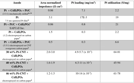
composites result in uniformly distributed porous nanostructures. Table 1.2 details the progress of SAFC anodes in terms of performance, Pt loading and Pt utilization thus far.

Anode Area normalized

impedance (Ω cm2₎

Pt loading (mg/cm2_{) Pt utilization (S/mg)}

Pt + CsH2PO4 + Pt/C

(3:3:1) mechanically milled26, 30

0.06 7.1 2.2

Pt 7.5 nm sputtered Pt film31

3.1 17E-3 19

Pt + Pt/C + CsH2PO49

SAFCell Inc.

0.06 0.8 21

Pt + CsH2PO4

(1:2) electrosprayed on carbon paper7

1.5 0.3 2.2

Pt + CsH2PO4 + Pt/C

(3:3:1) electrosprayed on CNT overgrown carbon paper6

0.5 0.3 6.6

30 wt% Pt-CNT + CsH2PO4

electrosprayed on carbon paper8

2.0-3.0 4.9-5.7 (x 10-3_{) 64-81}

40 wt% Pt-CNT + CsH2PO4

electrosprayed on carbon paper8

1.6-1.9 6.3-11 (x 10-3_{) 45-94}

46 wt% Pt-CNT + CsH2PO4

electrosprayed on carbon paper8

1.2-1.3 10-14 (x 10-3_{) 61-78}

Table 1.2.Progress of Pt-CNT-CsH2PO4 SAFC anodes thus far

1.4. Objectives of this thesis

Alternative cathode catalysts- The oxygen reduction reaction (ORR) at the cathode is the dominant contributor to the overpotential in fuel cell systems, and is therefore the focus of tremendous electrocatalysis research. Generally, the cathode requires higher catalyst loading in various energy conversion processes and the allure of replacing precious metal catalysts with alternatives to precious metal catalysts has garnered attention. This dissertation aims to access the efficacy of carbon nanostructures and oxides as oxygen reduction (ORR) reaction catalysts in solid acid fuel cells (SAFCs) cathodes.

C H A P T E R 2

Experimental methods

In this chapter, we introduce the underlying principles of the characterization techniques and the synthesis methods used in this work.

2.1. Characterization techniques

We can divide characterization techniques into two types: (a) Electrochemical characterization (in-situ) and (b) ex situ characterization. In situ techniques use the electrochemical variables of voltage, current and time to characterize the performance of fuel cell under operating conditions. (b) Ex situ techniques characterize the structure or chemical properties of fuel cell components employing methods such as Raman spectroscopy, x-ray photoelectron spectroscopy (XPS), and infrared spectroscopy. In this section, Raman spectroscopy is discussed.

2.1.1. Electrochemical characterization (in situ)

2.1.1.1 Current voltage (j-V) measurement

In the steady state j-V measurement, the current/voltage is held fixed in time and the steady state value of the fuel cell voltage/current is recorded after a long equilibration time. A high performance fuel cell will exhibit higher voltage for a given current load. By slowly stepping the current demand, the entire j-V response of the fuel cell can be recorded. For small fuel cell systems, a slow scan j-V curve can be recorded where the current demanded is gradually scanned in time from zero to a set limit and the voltage is recorded as it steadily drops. Alternatively, the voltage applied can be scanned in a predetermined range and the resulting current measured. To determine the suitable scan rate, a series of j-V curves at different scan rates should be measured first. If the scan rate is too fast, the j-V will be artificially high. The point at which the decreasing the scan speed no longer affects the j-V curve significantly is usually a good indication of a suitable scan rate.10

At low current densities as illustrated in Figure 1.1, ohmic losses can be calculated from Equation 1.3 and subtracted, and the approximate activation loss can be calculated from the data. If the j-V curve is plotted on a log scale, the low current density region shows linear behavior. In low-temperature fuel cells, reaction kinetics are slow and large activation potentials are required at both electrodes. Data analysis of the j-V curve by the Tafel equation allows approximate activation losses to be isolated. The Tafel equation can be written10

𝜂_𝑎𝑐𝑡 = 𝑅𝑇

𝑛𝛼𝐹ln(𝑗0) −

𝑅𝑇

𝑛𝛼𝐹ln(𝑗), (2.1)

where n is the number of electrons transferred in the redox reaction, jo is the exchange current

density, and α is the transfer coefficient. Experimental data plotted in the form η versus ln(j) can be fit with a line that yields a slope of α and intercept ln(j0) as illustrated in Figure 2.1a. From the

Tafel equation, it is evident that to lower ηact, larger values of α and j0 are desirable. To increase

the exchange current density (jo), the intrinsic activity of the catalyst needs to be improved or the

Figure 2.1. (a) The j-η representation of a hypothetical electrochemical reaction. The Tafel approximation deviates from Butler-Volmer kinetics at low overpotentials.10 (b) Effect of overpotential on fuel cell performance.

2.1.1.2. AC Impedance spectroscopy

Alternating current impedance spectroscopy is the study of microscopic processes simulated by an electric field. It is a widely used technique for fuel cell electrochemistry because it gives insight into material properties, transport processes and electrode | electrolyte interfacial processes.10, 32, 33 In an impedance measurement, a low sinusoidal voltage V(t) of varying frequency is applied to the system and the resulting current is measured. The current response will have the same frequency as the voltage perturbation but will generally have a phase shift as illustrated in Figure 2.2a. The frequency variation in voltage gives insight into different electrochemical processes in the system with a characteristic timescale. In comparison to a fuel cell measurement, a small signal voltage perturbation confines the impedance measurement to a pseudo-linear portion of a fuel cell’s I-V curve as shown in Figure 2.2b.10

Figure 2.2. (a) Application of a small signal perturbation confines the impedance measurement to a pseudo-linear portion of a fuel cell’s I-V curve (b) A sinusoidal voltage perturbation and resulting current response with a phase shift (θ)

The input signal is a complex time-dependent wave function of the form

𝑉(𝑡) = 𝑉₀∙ 𝑒𝑗𝜔𝑡_{, (2.2)}

where V0 is the amplitude voltage, the angular frequency ω = 2πf and j is the complex index. For

a small voltage perturbation, this input potential generates a current output;

𝐼(𝑡) = 𝐼₀∙ 𝑒𝑗(𝜔𝑡+𝜃), (2.3)

where θ is the phase shift. The respective impedance Z is calculated as

𝑍(𝑤) =𝑉(𝑡)

𝐼(𝑡) = |𝑍|𝑒

−𝑗𝜃 _{= |𝑍| cos(𝜃) − 𝑗|𝑍| sin(𝜃) = 𝑍}

𝑅𝑒 − 𝑗𝑍𝐼𝑚, (2.4)

where ZRe is the real and ZIm is the imaginary part of the impedance and |Z| is the impedance

modulus.32, 33

electrochemical processes with sufficiently different characteristic timescales (at least two orders of magnitude apart) can be distinguished as separate arcs along the real axis. Another common representation is the Bode-Bode plot, which is a plot of |Z|(ω) versus θ(ω), where |Z| and θ are

|𝑍| = 𝑍(𝜔) = √𝑍_𝑅2 _{+ 𝑍}

𝐼2, (2.5)

𝜃 = 𝑡𝑎𝑛−1₍𝑧𝐼

𝑍𝑅). (2.6)

Figure 2.3a shows the Nyquist plot of a hypothetical fuel cell. For the hypothetical fuel cell, the

size of these two semicircles, ZA and ZC, can be attributed to the magnitude of the anode and

cathode activation losses, respectively. The anode and cathode half reactions are shown in Figure 2.3b. ZΩ corresponds to ohmic losses across the electrolyte. In this hypothetical fuel cell, cathode

activation losses dominate fuel cell performance while anode activation and ohmic losses are small. This is the case for many fuel cell types.9, 10, 13, 34

Figure 2.3. (a) Nyquist plot of a hypothetical fuel cell. Regions marked correspond to ohmic, anode activation and cathode activation losses, respectively. (b) Schematic of a fuel cell with cathode and anode half reactions.

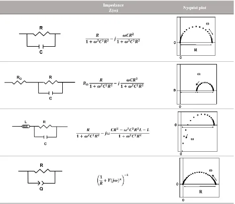
lattice and have a finite impedance. At lower frequencies the interaction of the charged species with grain boundaries can be sampled, and at even lower frequencies the electrode | electrolyte interface can be sampled. The impedance of each of these electrochemical processes can be modelled as a resistor and capacitor in parallel as shown in Figure 2.4c. The capacitor describes the charge separation between ions and electrons across the interface. The resistor describes the kinetic resistance to the electrochemical reaction process.10 At infinitely low frequencies, the impedance measured correspond to the resistance of all the processes in the system. Bulk processes typically have higher characteristic frequencies than electrode processes, hence yield arcs that are well separated from electrode arcs.3

Figure 2.4. (a) An illustration of the movement of a proton under electric field perturbation at varying frequencies. (b) Physical representation of an electrochemical interface. (c) Proposed equivalent circuit model of an electrochemical reaction interface.