HAAR Cascade Based Dynamic Traffic Scheduling System

5

VIII

August 2017

HAAR Cascade Based Dynamic Traffic Scheduling

System

Rishabh Sachdeva1, Sricheta Ruj2

1_{Computer Engineering, Shri Govindram Seksaria Institute of Technology and Science} 2_{Computer Engineering, Nirma University}

Abstract: Object Detection has become an important feature in field of Computer Science. Benefits of object detection are varied and are not restricted to any specific area. Instead, object detection technique is growing rapidly and used widely in Information Industry. This paper intends to address one such possibility with the help of Haar-cascade classifier. The focus of the paper will be on the case study to develop a Smart and Dynamic Traffic Management System which is based on vehicle detection mechanism.

Keywords: Haar cascades, OpenCV, Pixel, Image Feature, Adaboost

I.INTRODUCTION

A. Digital Image Processing

An image may be defined as two dimensional entity F(x,y), where x and y are spatial coordinates, and the amplitude of Function F at any pair of coordinates x,y is called intensity or gray level of image. When x, y and amplitude values of function F are finite and discrete entities, we call image a digital image.

The field of digital image processing refers to processing digital images by means of digital computer. A digital image is composed of finite number of elements, each of which has a particular location and value. These elements are referred to as picture elements, image elements and pixels.

B. RGB and Gray Scale Image

RGB (red, green, and blue) refers to a system for representing the colours to be used on a computer display. Red, green, and blue can be combined in various proportions to obtain any colour in the visible spectrum. Levels of R, G, and B can each range from 0 to 100 percent of full intensity. Gray scale images are distinct from one-bit bi-tonal black-and-white images, which in the context of computer imaging are images with only the two colours, black, and white (called bi-level or binary images) [1].

II. HAARCASCADES

Fig. 1 Image Features

III.FEATURECALCULATIONBYINTEGRALIMAGE

Integral image is an intermediate result of an image. This is used to determine rectangular features in the image. The integral image is generated from original image to make further process faster. Integral image is used to felicitate quick feature detection. It is the outline of the pixel values in the original image. The integral image at any location (coordinates x,y) is determined by adding the pixels above and to the left of coordinates x and y [2].

( , ) = ( , )

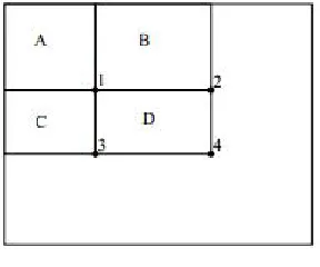
Consider I as integral image and O as original image. Referring Fig 2, value of integral image at point 1, is the total summation of pixels in Area A. At point 2, value is pixel summation of area A and area B. Similarly, at location 4 values is A+B+C+D. The pixel sum within D can be calculated as 4 - (2+3) - 1. So, the features are calculated by subtracting pixel values in different rectangles. To compute edge features (Figure 1), six array references are considered, eight in the case of line features and nine in the case of four-rectangle features. Then, this value is compared with desired criteria threshold to judge whether the window object is desired one or not.

Fig. 2 Array references

IV.ADABOOST

AdaBoost (Adaptive Boosting) is a machine learning meta-algorithm formulated by Freund and Schapire [3] was the first practical boosting algorithm, and remains one of the most widely used and studied, with applications in numerous fields. Adaboost is a technique that helps in combining number of “weak classifiers” into a single “strong classifier”. AdaBoost is adaptive in the sense that subsequent weak learners are tweaked in favour of those instances misclassified by previous classifiers. There is a standard characteristic of a weak classifier that it should have the detection rate of at least 50 per cent, .i.e. it should be able to detect at least half of the desired objects in an image. So, a bunch of trained classifiers can be used to develop an effectively trained mechanism to detect objects using Adaboost training mechanism. Following analysis is based on [3], [4] and [5].

A. Selection of Training Sets

examples so that these examples will make up a larger part of the next classifiers training set, and the next classifier trained will perform better on them.

B. Classifier Output Weights

After training of classifiers, the weight of each classifier is computed based on its accuracy. Classifiers that are more accurate are assigned more weight. Weighted classifiers are assigned more priority in determining results.

C. Definition and Equations

H(x) = αh (x)

The final classifier consists of T weak classifiers. h (x) is the output of weak classifier ‘t’. In this paper, outputs are limited to +1 or -1.α is the weight assigned to classifier t as determined by AdaBoost. The final output H is the linear summation of all the weak classifiers.

The classifiers are trained one at a time. After training of each classifier, probabilities of each of the training examples are updated for the next classifier. The first classifier (t=1) is trained with examples which all have equal probability. For output weight calculation of each classifier, following formula is used.

=1

2ln

1−

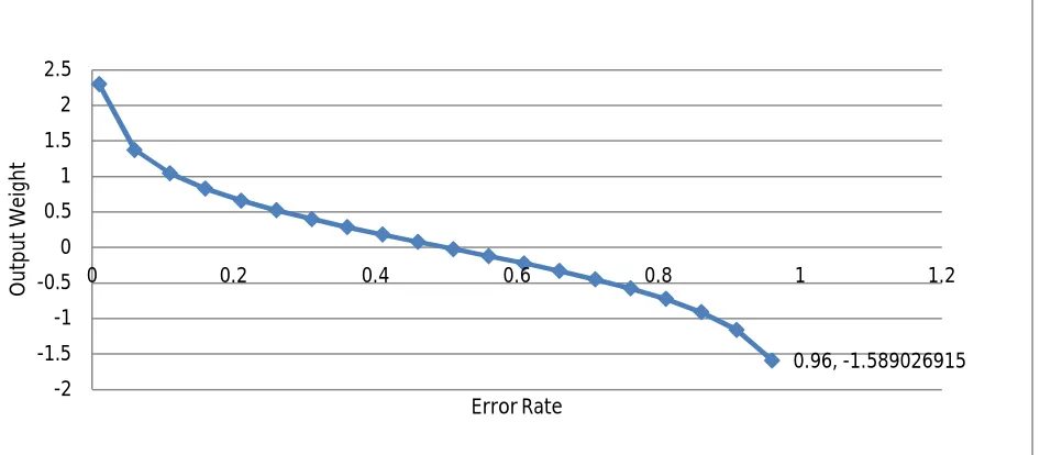
Formula for output weight is based on classifier’s error rate. is the number of misclassification over the training set divided by the total size of training set.[4]

Fig. 3 Output weight vs Error rate

Following points should be noted from the above graph.

1) The weight of classifier grows exponentially when erroe rate tends to 0. 2) The weight of classifier is 0 when error rate is 0.5 .

3) The weight of classifier grows exponentially negative when error rate approaches one. Those classifiers with error rate greater that 0.5 are no better than random guessing.

After computing at, training example weights are updated using following formula:

( ) = ( ) ( ) 0.96, -1.589026915 -2 -1.5 -1 -0.5 0 0.5 1 1.5 2 2.5

0 0.2 0.4 0.6 0.8 1 1.2

The variable is a vector of weights, with one weight for each training example in the training set. ‘ ’ refers to training example number. refers to distribution. Each weight ( ) represents the probability that training example ‘ ’ to be selected as part of the

training set. Weights are normalized by dividing each of them by sum of all the weights ( ).This vector is updated for each new

weak classifier that is trained. refers to the weight vector used when training classifier ‘t’. This equation needs to be evaluated for each of the training samples ‘ ’( , ). Each weight from the previous training round is going to be scaled up or down by this exponential term.The function will return a fraction for negative values of x, and a value greater than one for positive values of x. So the weight for training sample ‘ ’ will be either increased or decreased depending on the final sign of the term “− ∗ ∗ ℎ( )”. For binary classifiers whose output is constrained to either -1 or +1, the terms and ℎ( ) only contribute to the sign and not the magnitude.

is the correct output for training example ‘ ’, and ℎ ( ) is the predicted output by classifier t on this training example. If the predicted and actual outputs agree, ∗ ℎ( ) will always be +1 (either 1 * 1 or -1 * -1). Else, ∗ ℎ( ) will be a negative term. Ultimately, misclassification by a classifier with a positive (output weight) will result in giving this training example a larger weight.

Note: By introducing (output weight) in above formula, classifier’s effectiveness is also taken into consideration when updating weights.

A much more in-depth explanation of Adaboost algorithm can be found in a book by Schapire and Freund[6].

V. APPLICATIONINDYNAMICTRAFFICMANAGEMENTUSINGOPENCV

This section is devoted to the description of proposed vehicle detection system and management traffic system to make everyday life easier. This application uses Adaboost algorithm (described in section IV) to train classifiers for vehicle detection.

OpenCV (Open Source Computer Vision Library) is released under a BSD license and hence it’s free for both academic and commercial use. In this paper, we will use OpenCV to implement cacades and detect objects. The system is composed of three parts: learning section, detection section and traffic light management section.

A. Learning Section

This sections consists of two phases: Extraction phase and Training phase

1) Extraction Phase: In this phase, descriptor based on haar wavelet [7] extracted for each image in training set, a feature vector. This database contains set of positive samples (containing vehicle) and negative samples (containing no vehicle). Negative images should contain pictures, which can be found near vehicles on roads like grass, sign boards, road sign and hoarding boards. The negative image database helps training classifiers to ignore such windows containing such images and save time and hence making operation effective and less expensive.

Positive samples are created by using opencv_createsamples application. Bunch of positive samples can be created using this utility of OpenCV. It takes one object image in input and creates a large set of positive samples from the given object image by randomly rotating the object, changing the image intensity as well as placing the image on arbitrary backgrounds. However, considering only one image of vehicle is not a good idea. To create a robust system, large number of vehicles images of various categories is required. Following is the command to run create_sample utility:

Opencv_createsamples.exe –info <pathOfFileInfo.txt > -vec <vecFileName>

Output of above command is in form of vector file (.vec). Info.txt contains location positive sample images following the coordinates of bounding rectangle as mentioned below.

rawdata/positiveImages/pic1.bmp 1 80 73 86 176 rawdata/positiveImages/pic2.bmp 1 114 116 84 218

2) Training Phase: The next step is the actual training of the boosted cascade of weak classifiers, based on the vector file that was prepared in extraction phase. This where AdaBoosting (section IV) comes into picture. Internally, OpenCV uses boosting to train classifiers. The following command is used:

opencv_traincascade.exe data classifier vec <vecFileName> bg <PathOfNegative.txt> numStages 7 miniHitRate 0.98 -maxFalseAlarmRate 0.5

numStages refers to number of cascade stages to be trained. More details of parameters are present in [8]. Negative.txt contains location of negative image samples as shown below.

After the opencv_traincascade application has finished its work, the trained cascade will be saved in cascade.xml file in the -data folder. The commands mentioned above with additional parameters are present in detail in official website of OpenCV [8]. 3) Object Detection Section: The trained classifier generated in training phase (cascade.xml) is used to detect desired object. The

cascade.xml is loaded into detection program, image is passed as input, converted into gray scale image and finally program returns the position of detected object as Rectangle (x,y,w,h). Further, the count of objects detected is used in next stage.

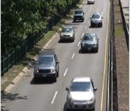
Fig. 4 Original Frame

Fig. 5 Vehicle tracking

Fig. 6 Flow diagram for traffic scheduling system

VI.CONCLUSION

Traffic congestion is a severe problem and the widespread use of information technology provides an opportunity to enhance the techniques of Traffic Management systems. This paper proposes a solution to achieve this via dynamic traffic scheduling. The image is first captured of a particular traffic lane from a traffic square. Then the adequate time duration is allotted to that lane for vehicle passage according to traffic density. There is always some threshold and maximum duration.Concept of Haar Cascade is used in implementation of classifiers and object detection. Haar Cascades based on Adaboost is used in this paper to train classifiers, which is further used to detect vehicles. AdaBoost, short for "Adaptive Boosting", is a machine learning meta-algorithm that helps in combining multiple “weak classifiers” into a single “strong classifier”. The output of the other learning algorithms ('weak learners') is combined into a weighted sum that represents the final output of the boosted classifier. OpenCV (Open Source Computer Vision Library) provides utilities for implementation of trained classifiers using positive and negative image samples as dataset.

REFERENCES

[1] G. Jyothi, CH. Sushma, D.S.S. Veeresh.“Luminance Based Conversion of Gray Scale Image to RGB Image”. International Journal of Computer Science and

Information Technology Research. Vol. 3, Issue 3, pp: (279-283), Month: July - September 2015, Available at: www.researchpublish.com

[2] Monali Chaudhari#1 , Shanta sondur*2 , Gauresh Vanjare$3. “A review on Face Detection and study of Viola Jones method”. International Journal of

Computer Trends and Technology (IJCTT) – volume 25 Number 1 – July 2015

[3] Freund, Y., Schapire, R.E.: A decision-theoretic generalization of on-line learning and an application to boosting. Journal of Computer and System Sciences

55(1), 119–139 (1997)

[5] Robert E. Schapire .” Explaining AdaBoost”. Available at http://rob.schapire.net/papers/explaining-adaboost.pdf .

[6] Schapire, R.E., Freund, Y.: Boosting: Foundations and Algorithms. MIT Press (2012)

[7] Viola P, Jones M. Rapid object detection using a boosted cascade of simple features. In: Computer Vision and Pattern Recognition. CVPR 2001. Proceedings of

the 2001 IEEE Computer Society Conference on; Vol. 1, pp. I-511.

[8] http://docs.opencv.org/trunk/d7/d8b/tutorial_py_face_detection.htmlandhttp://docs.opencv.org/trunk/db/d28/tutorial_cascade_classifier.html