Effect of Elements, Order of Approximation and Gauss Quadrature Points in Finite Element Method for Study of Rectangular Waveguides

(1)

International Journal of Emerging Technology and Advanced Engineering

Website: www.ijetae.com (ISSN 2250-2459, ISO 9001:2008 Certified Journal, Volume 4, Issue 5, May 2014)

1

Effect of Elements, Order of Approximation and Gauss

Quadrature Points in Finite Element Method for Study of

Rectangular Waveguides

M.M. Nagare

1

, S.K Popalghat

2

1_{Department of Physics, MSS’s Arts, Science and Commerce College, Ambad, Jalna-431203, MS, India.}

2_{Research Center, Post Graduate Department of Physics, JES College Jalna-421203, MS, India.}

Abstract— The main objective of this paper is to study the effect of number of elements, order of approximation and gauss quadrature points in finite element method for rectangular waveguide, which is the level at which the engineer is most interested in. By discretizing the cross-section of the waveguide into a number of rectangular elements, an eigenvalue problem is solved and electric field is plotted. Results are compared to analytical solutions and convergence of solution with increase in number of element, order of approximation and gauss points are clearly shown in graphs.

Keywords— Finite element, Waveguide, Microwave, Rectangular element, Order of approximation, Gauss point, FEM.

I. INTRODUCTION

The Finite Element Method (FEM) has been widely used in electromagnetic problem because it is an effective and accurate numerical method that is suitable for complex structures and material properties. The accuracy of solution in finite element method is depends upon discretization of mesh, order of approximation of shape functions and Gauss quadrature points used for line, surface and volume integration.

In Finite element method, the domain has to discretize with finite element such as Delaunay triangulation (for complex structure), but this paper is deal with the regular domain (Rectangular Waveguide) and hence rectangular element has been used in this study. Many researchers have developed numerical technique to study the numerical solution for regular as well as irregular domain [1,2,3,4]. Emphasize made in this work, to study the effect of elements, order of approximation and gauss quadrature points in finite element method to study the rectangular waveguides. In this work finite element solver has been developed in Java and automatic mesh generation program in Flash. The problem of domain is homogeneous hallow rectangular waveguide used for X band for the range of frequency 2.2 to 12.4 GHz.

II. TWO DIMENSIONAL PROBLEM FORMULATIONS

For a homogeneous isotropic medium, the scalar

potential function satisfies the Helmholtz equation with

wave number

…1

This is a strong form of the scalar Helmholtz equation [1]. In a strong form, the unknown appears within the second order differential operator. To make the equation suitable for numerical solution, it can be converted into ―Weak‖ form by multiplying both side with a test function

and by integrating over the surface ; that is

….2

First term of equation 2 can be written as

…3

The following vector identities can be used to modify equation 3

…4

And …5

Equation 2 can be now written as

… 6

Where is the normal derivative of along the

boundary the term on the right hand side vanishes

because for PEC boundary, =0 for TM mode and

(2)

International Journal of Emerging Technology and Advanced Engineering

531

Hence, equation 6 can be written as,

…7

This is the weak form.

III. DISCRETIZATION

The problem domain is discretized with the rectangular element with the help of mesh generation program written

in as2 script in Flash. The purpose to use flash is the

simplest way to manipulate rich graphics.

IV. SHAPE FUNCTION

Where p is the order of approximation, k is the element

number, i and j are node numbers. This one dimensional

shape function can be used to generate two dimensional rectangular shape functions by taking tensor product [1]

Pros: Extremely easy to determine the interpolating polynomial.

Cons: Lagrangian form of the polynomial more expensive to evaluate than monomial form. Also more difﬁcult to integrate, differentiate, etc.

In the standard Galerkin method, test function is

and approximate function is

… 10

If we put these values in equation 7, the system of linear equation is achieved, which in matrix form can be written as

…11

Where called as stiffness

matrix and called as mass matrix

After assembling, equation 11 becomes

… 12

Where K and M are global matrices of order

where n is the total number of nodes.

Equation 12 is generalized eigenvalue equation which is

solved for in MFEM, with the help of jblas.jar linear

algebra pack for java (Originally developed by Mikio L.

Braun) [18] . The cutoff wave number is given by .

V. FIELD COMPUTATION FROM SCALAR POTENTIAL

Once the scalar potential is calculated at every node, the electric field could be calculated for both TE and TM modes by the following formulation [1].

…13

And

…14

VI. BOUNDARY CONDITIONS:TEMODES

For TE modes, represents the axial magnetic field, Hz,

and the boundary condition is the Neumann

condition , where n is normal to the perfectly

conducted boundary [4]. In FEM, this is a natural boundary condition and need not be imposed. Thus, the Values at the boundary are considered to be unknown and the eigenvalue equation (12) is solved using the MFEM.

VII. BOUNDARY CONDITIONS:TMMODES

For TM modes, represents the axial electric field Ez,

and the boundary condition for the perfectly conducted

boundary is, = 0. This is the Dirichlet condition, which must be strictly imposed in the FEM. It can be done by

(i) Omitting differentiation with respect to the known boundary nodes. This can be done by simply deleting the

rows of Stiffness and Mass matrices corresponding to the

boundary nodes. This technique will reduce the dimension of Global matrices.

(3)

International Journal of Emerging Technology and Advanced Engineering

532

VIII. NUMERICAL RESULT AND DISCUSSION

Rectangular Waveguide

The cutoff frequency and field distribution for TE10 and TE20 modes for hallow rectangular waveguide of dimension a=2.4 cm and b=1.2 cm is calculated and result is compared with analytical value. The convergence of

solution assessed with element effect, order of

approximation and gauss points are shown in tables. The

exact value of TE10=6.245676 GHz and

[image:3.612.89.243.270.355.2]

TE20=12.491352GHz [17].

[image:3.612.318.570.319.692.2]

Figure 1 Dimension of hallow rectangular waveguide

Figure 2 Rectangular mesh generated in flash

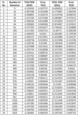
For the order of approximation 1 and gauss points 3, the cutoff frequency and error of first two dominant modes, TE10 and TE 20 are calculated by increasing elements from 9 to 3025 as shown in table 1.

It is observed that, solution converges to exact solution for more than 400 elements for first order approximation.

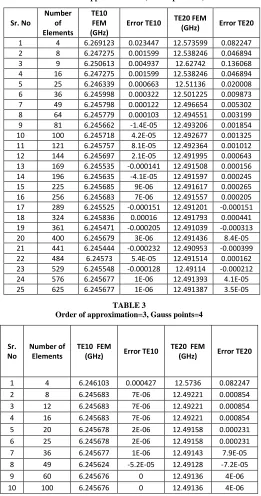
For the order of approximation 2 and gauss points 3, the cutoff frequency and error of first two dominant modes TE10 and TE20 are calculated by increasing elements from 4 to 625 as shown in table 2 and it observed that solution converges for more than 25 elements.

For the order of approximation 3 and gauss point 4, the cutoff frequency and error of TE10 and TE20 are calculated by increasing elements from 4 to 100 and it observed that solution converges very rapidly only from eight elements.

From tabulated values it clear that, TE20 mode required more element than TE10 mode for all order of approximation.

While doing work, surprising thing has been observed in numerical surface integration, which is stated as follows.

Theoretically it is well known that, any polynomial of

order 2 can be integrated exactly using nth order

gauss quadrature [5], it means that for 2 gauss quadrature

points 3rd order polynomial would have given exact answer

and there would have no problem in getting finite element answer in solver.

But while studying effect of gauss quadrature points in solution, it is observed that, for degree of polynomial n, the minimum required gauss quadrature points are n+1.

Less than above condition will cause non positive definite mass matrix.

TABLE 1

Order of Approximation=1, Gauss Points=3

Sr. No

Number of Elements

TE10 FEM (GHZ)

Error TE10

TE20 FEM (GHz)

Error TE20

1 9 6.533433 0.287757 14.609201 2.117849

2 16 6.407184 0.161508 13.773687 1.282335

3 25 6.348855 0.103179 13.319728 0.828376

4 36 6.317244 0.071568 13.066867 0.575515

5 49 6.298164 0.052488 12.913629 0.422277

6 64 6.285882 0.040206 12.814367 0.323015

7 81 6.277353 0.031677 12.746161 0.254809

8 100 6.271391 0.025715 12.69771 0.206358

9 121 6.266976 0.0213 12.661891 0.170539

10 144 6.263527 0.017851 12.634489 0.143137

11 169 6.260728 0.015052 12.612948 0.121596

12 196 6.258736 0.01306 12.596328 0.104976

13 225 6.257098 0.011422 12.582864 0.091512

14 256 6.255714 0.010038 12.571763 0.080411

15 289 6.254411 0.008735 12.562253 0.070901

16 324 6.253763 0.008087 12.555177 0.063825

17 361 6.252585 0.006909 12.547927 0.056575

18 400 6.252099 0.006423 12.542782 0.05143

19 441 6.251268 0.005592 12.537526 0.046174

20 484 6.251036 0.00536 12.533952 0.0426

21 529 6.250402 0.004726 12.529969 0.038617

22 576 6.250136 0.00446 12.527055 0.035703

23 625 6.249787 0.004111 12.524254 0.032902

24 676 6.24932 0.003644 12.521457 0.030105

25 729 6.249122 0.003446 12.5194 0.028048

26 784 6.249265 0.003589 12.518203 0.026851

27 841 6.248627 0.002951 12.51559 0.024238

28 900 6.24853 0.002854 12.514195 0.022843

29 961 6.248297 0.002621 12.51264 0.021288

30 1024 6.248185 0.002509 12.511428 0.020076

31 1600 6.247282 0.001606 12.504199 0.012847

32 2025 6.247335 0.001659 12.502283 0.010931

33 2500 6.246704 0.001028 12.499573 0.008221

[image:3.612.77.259.381.488.2]

(4)

International Journal of Emerging Technology and Advanced Engineering

[image:4.612.323.581.151.296.2]

533

TABLE 2

[image:4.612.39.300.152.648.2]

Order of approximation=2, Gauss points=3,

TABLE 3

Order of approximation=3, Gauss points=4

Sr. No

Number of Elements

TE10 FEM

(GHz) Error TE10

TE20 FEM

1 4 6.246103 0.000427 12.5736 0.082247

2 8 6.245683 7E-06 12.49221 0.000854

3 12 6.245683 7E-06 12.49221 0.000854

4 16 6.245683 7E-06 12.49221 0.000854

5 20 6.245678 2E-06 12.49158 0.000231

6 25 6.245678 2E-06 12.49158 0.000231

7 36 6.245677 1E-06 12.49143 7.9E-05

8 49 6.245624 -5.2E-05 12.49128 -7.2E-05

9 60 6.245676 0 12.49136 4E-06

10 100 6.245676 0 12.49136 4E-06

IX. GRAPHS

5.8 6 6.2 6.4 6.6 6.8 7

4 ₁₆ ₃₆ ₆₄

100 144 196 256 324 400 484 576 676 784 900 ₁₀₂4 ₂₀₂5 ₃₀₂5

F r e q u e n c y

G H Z

Elements

[image:4.612.42.300.158.653.2]

TE10 Exact TE10 FEM

[image:4.612.321.579.328.456.2]

Figure 3 Convergence of solution as element increases for TE10 mode for first order approximation

Figure 4 Convergence of solution as element increases for TE20 mode for first order approximation

Figure 5 Convergence of solution as element increases for TE10 mode for second order approximation

Sr. No

Number of Elements

TE10 FEM (GHz)

Error TE10 TE20 FEM

1 4 6.269123 0.023447 12.573599 0.082247

2 8 6.247275 0.001599 12.538246 0.046894

3 9 6.250613 0.004937 12.62742 0.136068

4 16 6.247275 0.001599 12.538246 0.046894

5 25 6.246339 0.000663 12.51136 0.020008

6 36 6.245998 0.000322 12.501225 0.009873

7 49 6.245798 0.000122 12.496654 0.005302

8 64 6.245779 0.000103 12.494551 0.003199

9 81 6.245662 -1.4E-05 12.493206 0.001854

10 100 6.245718 4.2E-05 12.492677 0.001325

11 121 6.245757 8.1E-05 12.492364 0.001012

12 144 6.245697 2.1E-05 12.491995 0.000643

13 169 6.245535 -0.000141 12.491508 0.000156

14 196 6.245635 -4.1E-05 12.491597 0.000245

15 225 6.245685 9E-06 12.491617 0.000265

16 256 6.245683 7E-06 12.491557 0.000205

17 289 6.245525 -0.000151 12.491201 -0.000151

18 324 6.245836 0.00016 12.491793 0.000441

19 361 6.245471 -0.000205 12.491039 -0.000313

20 400 6.245679 3E-06 12.491436 8.4E-05

21 441 6.245444 -0.000232 12.490953 -0.000399

22 484 6.24573 5.4E-05 12.491514 0.000162

23 529 6.245548 -0.000128 12.49114 -0.000212

24 576 6.245677 1E-06 12.491393 4.1E-05

[image:4.612.332.556.488.622.2]

(5)

International Journal of Emerging Technology and Advanced Engineering

534

12.48 12.5 12.52 12.54 12.56 12.58 12.6 12.62 12.64

0 100 200 300 400 500 600 700

F r e q u e n c y

G H Z

Elements

[image:5.612.51.297.132.277.2]

TE20 Exact TE20 FEM

Figure 6 Convergence of solution as element increases for TE20 mode for second order approximation

6.2456 6.2457 6.2458 6.2459 6.246 6.2461 6.2462

0 20 40 60 80 100 120

F r e q u e n c

y G H Z

Elements

[image:5.612.331.555.181.577.2]

TE10 Exact TE10 FEM

Figure 7 Convergence of solution as element increases for TE10 mode for third order approximation

Figure 8 Convergence of solution as element increases for TE20 mode for third order approximation

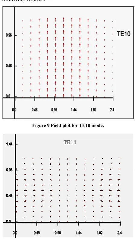
X. ELECTRIC FIELD DISTRIBUTION IN RECTANGULAR WAVEGUIDE

First four modes of electric field plots have been shown in following figures.

[image:5.612.50.297.315.450.2]

Figure 9 Field plot for TE10 mode.

[image:5.612.51.288.475.599.2]

(6)

International Journal of Emerging Technology and Advanced Engineering

[image:6.612.60.277.114.586.2]

535

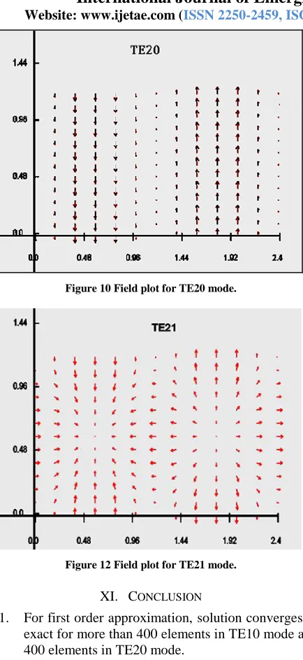
[image:6.612.316.566.138.679.2]

XI. CONCLUSION

1. For first order approximation, solution converges to

exact for more than 400 elements in TE10 mode and 400 elements in TE20 mode.

2. For second order approximation, solution converges

rapidly for more than 16 elements in TE10 mode and more than 58 elements in TE20 mode.

3. For third order approximation, solution converges

on more than 4 elements in TE10 mode and more than 8 elements in TE20 mode.

4. The minimum required gauss quadrature points for

finite element method are for nth order of

polynomial shape functions. Above this, there is no effect found in accuracy of solution, and less than this, causes non positive definite mass matrix.

REFERENCES

[1 ] Reddy, C. J, Manohar D. Deshpande, C. R. Cockrell, and Fred B. Beck, ―Finite Element Method for Eigenvalue Problems in Electromagnetics‖ NASA Technical Paper 3485, 1994.

[2 ] Liu J. and Lin G. ― Analysis of a Quadruple Corner-Cut Ridged/Vane-Loaded Circular Waveguide using Scaled Boundary Finite Element Method‖ Progress In Electromagnetics Research M, Vol. 17, 113-133, 2011.

[3 ] Vaish A. and Parthasarathy H ― Analysis of a Rectangular Waveguide using Finite Element Method‖ Progress In Electromagnetics Research C, Vol. 2, 117–125, 2008

[4 ] Rahaman, B.M.A, ―Finite Element Analysis of Optical Waveguide‖ progress in Electromagnetic Research, PIER 10, 187-216, 1995. [5 ] Uppadhay, C.S, ―Mechanical - Finite Element Method‖ by nptelhrd ,

Department of Aero Space IIT Kanpur 2013. URL: http://www.youtube.com/view_play_list?p=A4CBD0C55B9C3878 [6 ] Haldar, M. K, ―Introducing the Finite Element Method in

electromagnetics to undergraduates using MATLAB, Department of Electrical and Computer Engineering, National University of Singapore.

[7 ] Peter J. Olver "Finite Element method", 2012

[8 ] Lifang Wang, "Convex Mesh free Solution for arbitrary Waveguide Analysis in electromagnetic Problems" Progress In Electromagnetics Research B, Vol. 48, 131149, 2013.

[9 ] Hopfer S, ‗Design of Ridged Waveguides‘, IRE Trans. Microwave. Theory. Tech., 3 (1955), 20–29.

[10 ]Helszain, J, ―Ridge Waveguides and Passive Microwave Components.‖ Published by the institute of engineering and technology, London, United Kingdom 2000.

[11 ]Francisco-Javier Sayas "A gentle introduction to the Finite Element Method"2008.

[12 ]Germund Dalquist and Ake Bjorck "Numerical Methods in Scientific Computing, Volume1" Siam, Socity for Industrial and applied Mathematics 3600 Market Street, 6 th floor, Philadelphia 2008.

[13 ]Reddy, J.N, "An Introduction to the Finite Element Method" McGraw-Hill Book 1984.

[14 ]Pelosi, Giuseppe. Quick Finite Elements for Electromagnetic Waves (2nd Edition), 2009. http://site.ebrary.com/id/10359080?ppg=19 [15 ]Keith W. Whites, ―Laboratory for Applied Electromagnetics and

Communications Department of Electrical and Computer Engineering South Dakota School of Mines and Technology‖. 2013 [16 ]Liu, G. R. ―Finite Element Method: A Practical Course‖.

http://site.ebrary.com/id/10169772?ppg=7, 2013.

[17 ]Pozar D.M ―Microwave Engineering -4th editions‖ Copyright C_ 2012, 2005, 1998 by John Wiley & Sons, Inc.