BIROn - Birkbeck Institutional Research Online
Adam, S.P. and Karras, D.A. and Magoulas, George D. and Vrahatis, M.N.
(2015) Reliable estimation of a neural network’s domain of validity through
interval analysis based inversion. In: 2015 International Joint Conference on
Neural Networks (IJCNN), 12-17 July 2015, Killarney.
Downloaded from:
Usage Guidelines:
Please refer to usage guidelines at
or alternatively
Reliable estimation of a neural network’s domain of
validity through interval analysis based inversion
S. P. Adam
∗, D. A. Karras
†, G. D. Magoulas
‡and M. N. Vrahatis
§ ∗Computational Intelligence Laboratory, Department of Mathematics, University of Patras,GR-26110 Patras, Greece. Email: [email protected] and
Department of Computer Engineering, Technological Educational Institution of Epirus, 47100 Arta, Greece.
†Department of Automation, Technological Educational Institution of Sterea Hellas,
34400 Psahna, Evia, Greece. Email: [email protected]
‡Department of Computer Science and Information Systems, Birkbeck College, University of London,
Malet Street, London WC1E 7HX, United Kingdom. Email: [email protected]
§Computational Intelligence Laboratory, Department of Mathematics, University of Patras,
GR-26110 Patras, Greece. Email: [email protected])
Abstract—Reliable estimation of a neural network’s domain of validity is important for a number of reasons such as assessing its ability to cope with a given problem, evaluating the consistency of its generalization etc. In this paper we introduce a new approach to estimate the domain of validity of a neural network based on Set Inversion Via Interval Analysis (SIVIA), the methodology established by Jaulin and Walter [1]. This approach was originally introduced in order to solve nonlinear parameter estimation problems in a bounded error context and proved to be effective in tackling several types of problems dealing with nonlinear systems analysis. The dependence of a neural network output on the pattern data is a nonlinear function and hence derivation of the impact of the input data to the neural network function can be addressed as a nonlinear parameter estimation problem that can be tackled by SIVIA. We present concrete application examples and show how the proposed method allows to delimit the domain of validity of a trained neural network. We discuss advantages, pitfalls and potential improvements offered to neural networks.
I. INTRODUCTION
Feed-forward neural networks are trained to form a mapping capable to model a process known through a set of data sampled from this process. This mapping is done in terms of realizing a functionF(x, w)that is close enough to a target function d =f(x) representing the underlying process. This target function is rarely formulated in analytical terms but it is defined as a set of input-output values {xi, di} resulting
from observations of the underlying process. Training a neural network is carried out by fixing the inputxiand outputdiand
adjusting the weights w until some distance metric between the realized and the target function is minimized.
It is well known in the neural network research community that a properly trained neural network is capable of modeling the underlying process when it is able to provide reliable generalization response i.e. correct classification of previously unseen data. Generalization depends not only on the training algorithm itself, but also, on both the training set and the location of the chosen validation points with respect to the area in the pattern space containing the set of training points. In consequence, it is necessary to be able to accurately
estimate the neural network’s domain of validity [2]. Another key issue for efficiently using a neural network concerns its ability to provide explanation on how it solves a particular problem especially when this deals with classification. As in the case of generalization, the ability to have an accurate estimation of the domain of validity is mandatory for deriving provably correct rules of the network’s classification function. Since the early times of neural research, a common approach to tackle these problems has always been neural network inversion. Before, getting into describing the details of neural network inversion we need to mention the work of Courrieu [2] and Pellilo [3] who study in depth algorithmic solutions for estimating the domain of validity of a neural network.
Typically, the term inversion corresponds to defining the inverse of the mapping F : Rn → Rm established by
a trained neural network, that is, the mapping denoted by
F−1:Rm→Rn. Given that theF is, generally, not invertible
in the classical sense F−1 is usually a one-to-many mapping which clearly defines neural network inversion as an ill-posed problem. Inversion methods proposed in the literature aim in defining the network input giving the best possible fit to one or more output values.
Several algorithms for inverting feed-forward neural networks have been proposed so far. A survey on these algorithms and related applications can be found in [4]. The authors of this paper formulate the inversion problem, analyze a number of techniques for solving this problem and present applications validating these techniques. Moreover, they propose the following broad areas for classifying the inversion methods: exhaustive search, single element search and population-based/evolutionary methods.
and Marks [8]. Given the manifold described by F(x) = y0,
where y0 is a predefined output level, x is an input vector
and F is the function implemented by the trained neural network, the method seeks to evenly distribute points on this surface. The method proposed by Jordan and Rumelhart [9] uses two neural networks, one for learning the direct mapping and a second one connected in series with the previous. The composite network is trained to learn an identity mapping and so the second network gives a particular inverse mapping of the direct one. Lu et al. [10] use mathematical programming techniques, such as linear and nonlinear programming based on the type of network to be inverted or the type of inversion to be performed. Also, it is worth mentioning the approach HYPINV proposed in [11] by Saad and Wunsch who use inversion in order to provide neural network explanation. HYPINV is a pedagogical algorithm, that extracts rules, in the form of hyperplanes.
Hereafter, let us present a few approaches built on the concept of interval. In [12] Thrun introduces Validity Interval Analysis (VI-Analysis) for extracting symbolic knowledge from feed-forward neural networks trained with a back-propagation algorithm. VI-Analysis “allows assertions to be made about the relation of activation values of a network by analyzing its weights and biases.” First, intervals are initialized with arbitrary values for all nodes, or some of them. Then, VI-Analysis refines these intervals by iteratively checking consistency of the activation values with the weights and the biases of the network. Thus, values found to be inconsistent are excluded. This is one of the first approaches attempting to analyze the input space by using the concept of interval while, however, being far from considering the concepts of Interval Analysis (IA).
Another approach using Interval Arithmetic to extract rules from feed-forward neural networks is described in [13]. This approach is calledDeep Thoughtand extracts rules from a trained multilayer perceptron in the form of intervals of activation, which input neurons can take so that a desired output is produced by the network. The authors state that intervals of activation are defined in a feed-forward manner which consists in “identifying the largest hypercube in the input space which will account for the desired output and then proceeds with space-fill the allowable input with successive smaller hypercubes until a stopping criterion is satisfied.” For the inverse operation “moving from output to input in the neural network” Simplex Optimization is used. Hence, it is clear that the proposed approach does not adopt the principles of IA especially as far as function evaluation is concerned. The complexity of the method is exponential with respect to the problem dimension i.e. the number of input neurons.
Finally, the algorithm developed by Hern´andez-Espinosa et al. [14] which consists in performing rule extraction based on Interval Arithmetic. This algorithm adopts the same principle with the approach of Kindermann and Linden [6], that is, to apply an iterative gradient descent algorithm in order minimize the error value by changing the initial input. The difference with this approach is that it considers interval valued inputs and computes the gradient using an interval version of gradient descent quite similar to one of the approaches proposed in [15].
The method presented in this paper builds exclusively on IA concepts and so it is completely different from the above presented methods. Starting from an interval which is the
range of the network output values it delivers a union of boxes containing the part of the input space whose image via the neural network mapping is the interval containing the output values. The method performs exhaustive search of the input space and so its efficiency depends on the dimensionality of the input and the range of each input variable. Despite these performance constraints our hypothesis is that a method that relies exclusively on IA concepts can effectively exploit the potential offered by IA methods and techniques. For instance, the fact that the output may be defined as an interval permits to consider those parts of the input space that contribute to the uncertainty of the network output.
The paper is organized as follows. Section 2 introduces the concepts from IA that are necessary for developing the proposed method. Section 3 describes how the method works to invert a feed-forward neural network, gives some application examples and related visualization of the inversion results. In Section 4 we discuss the advantages the pitfalls and the questions raised by this method. Finally, section 5 concludes the paper with some important remarks.
II. THEINTERVALANALYSISFORMALISM
A. Basic Concepts
The arithmetic defined on sets of intervals, rather than sets of real numbers is called interval arithmetic. An interval or interval number I is a closed interval [a, b] ⊂ R of all real numbers between (and including) the endpoints aand b, with a6b. The terms interval number and interval are used interchangeably. Whenever a = b the interval is said to be degenerate, thin or even point interval. Regarding notation, an interval x may be also denoted [x, x] or [x]or even [xL, xU]
where subscripts L andU stand for lower and upper bounds
respectively. Notation for interval variables may be uppercase or lowercase [16]. For the rest of this subsection let us denotex
an interval object (variable, vector, matrix, etc) to differentiate it from the explicit bracketed notation [x, x]. An interval
[x, x] where x = −x is called a symmetric interval. An n -dimensional interval vectorVis a vector havingncomponents
(v1,v2, . . . ,vn)such that every component vi,1 6i 6nis a
real interval [vi, vi]. Generally the following notation is used,
mid(x) = (x+x)/2, is the midpoint ofx, width(x) =x−x, is the diameter of the intervalx,
IR, denotes the set of real intervals, IRn, denotes the set ofn−dimensional
vectors of real intervals.
Let denote one of the elementary arithmetic operators
{+,−,×,÷} for the simple arithmetic of real numbers x, y. If x= [x, x] andy= [y, y]denote real intervals then the four elementary arithmetic operations are defined by the rule
x y={x y|x∈x, y∈y} (1)
each arithmetic operation:
x+y= [x+y, x+y] (2a)
x−y= [x−y, x−y] (2b)
x×y=
min xy, xy, xy, xy
,max xy, xy, xy, xy (2c)
x÷y=x×1
y,with (2d)
1
y =
1
y, 1 y
,provided that 0∈/
y, y
(2e)
Interval arithmetic operations are said to be inclusion isotonic
or inclusion monotonicor eveninclusion monotonegiven that the following relations hold,
if a,b,c,d∈IR and a⊆b,c⊆d (3)
then ac⊆bd, ∈ {+,−,×,÷}.
Let f : D ⊂ R → R be a real function and [x] ⊆ D
an interval in its domain of definition. The range of values of f over [x] may be denoted R(f; [x]) (see [16]) or simply
f([x]). Computing the rangeR(f; [x])of a real function by IA tools practically comes to enclosing the range R(f; [x])by an interval which is as narrow as possible. This is an important task in IA which can be used for various reasons, such as localizing and enclosing global minimizers and global minima of f on [x], verifying that R(f; [x]) ⊆ [y] for some given interval [y], verifying the nonexistence of a zero of f in [x]
etc.
Enclosing the range of f over an interval [x], f([x]), is achieved by defining a suitable interval function[f] :IR→IR
such that ∀[x] ∈ IR, f([x]) ⊂ [f]([x]), see Figure 1. This
interval function is called an inclusion function of f. What is important with an inclusion function [f] is that it makes possible to compute a box [f]([x]) which is guaranteed to containf([x]), whatever the shape off([x]), [17]. Note that the so-called natural inclusion function is defined if f(x), x∈D
is computed as a finite composition of elementary arithmetic operators {+,−,×,÷} and standard functions ϕ ∈ F as above. The natural inclusion function of f is obtained by replacing the real variable xby an interval variable[x]⊆D, each operator or function by its interval counterpart and evaluating the resulting interval expression using the rules in the previous paragraphs. The natural inclusion function has important properties such as being inclusion monotonic and if
f involves only continuous operators and continuous standard functions it is convergent, see [17].
B. The SIVIA approach
SIVIA was originally proposed by Jaulin and Walter [1] in order to provide guaranteed nonlinear parameter estimation from bounded error data. The objective of the method is to define a box or union of boxes enclosing a set of interest. More precisely, given a function f : X → Y
where X ⊂ Rn, Y ⊂ Rm and an interval vector (box) [y]⊆Y, the problem is to define the set of unknown vectors
x ∈ X such that f(x) ∈ [y], or in other words, define the set S ={x∈X ⊆Rn|f(x)∈ [y]} =f−1([y])∩X. In this
[image:4.612.326.553.60.192.2]definition X is the search space supposed to contain the set of interest S; [y] is a priori known to enclose the image of the set of interest f(S) and S denotes the unknown set of interest. Note that, f may not be invertible in the classical
Fig. 1:A functionf, an inclusion function[f]and the images of[x]
sense and hence f−1 simply denotes the reciprocal image of
f.
A solution to this problem consists in computing boxes or unions of boxes S− and S+ = S− ∪∆S that constitute
guaranteed outer and inner enclosures of S i.e. satisfying the relation S− ⊆ S ⊆ S+, [18]. SIVIA computes these
enclosures by recursively exploring the search space. It applies to any function f for which an inclusion function[f] can be computed. A box[x]∈Rn is designated as feasible if[x]∈S
and f([x]) ⊆ [y]. This condition is necessary and sufficient for [x] to be feasible. IA defines the conditions to decide the feasibility of a box [x]. Thus, if [f]([x]) ⊆ [y] then [x] is feasible otherwise if [f]([x])∩[y] =∅ then[x] is infeasible. In all other cases[x]is said to be indeterminate which means that [x]may be feasible, unfeasible or ambiguous.
Before calling SIVIA the following parameters need to be initialized; the box X which is guaranteed to enclose the set of interest S, an inclusion function [f] of the mapping
f and a lower limit ε for the width of the boxes covering
S. This parameter, ε, defines the precision that is acceptable for covering S. For any box[x] SIVIA examines if f([x]) is inside[y]. If this is true[x]then merges withS−else iff([x])
has no intersection with[y]then[x]∈/S and is rejected. If the width of [x] is less than the precision defined by ε then [x]
merges with ∆S, otherwise[x]is bisected and SIVIA restarts with the each one of the two sub-boxes. The algorithm below [18] gives a formal description of the method.
Algorithm 1 SIVIA(in:[x]; inout: S−,∆S)
Require: before calling SIVIA initialize f, [y] and ε;
S−← ∅;∆S← ∅;
1: if[f]([x])⊂[y]then
2: S−:=S−∪[x];
3: return;
4: end if
5: if[f]([x])∩[y] =∅then
6: return;
7: end if
8: ifwidth([x])< εthen
9: ∆S:= ∆S∪[x];
10: return;
11: end if
12: bisect[x]getting left and right sub-boxes[x]1 and[x]2
13: SIVIA([x]1,S−,∆S);
14: SIVIA([x]2,S−,∆S);
ability to back-up and load internal data in a simple format etc.
III. APPLYINGSIVIA
A. Assumptions
In this section we report how SIVIA is applied to specific problems and the results obtained. The experiments carried out concern the application of SIVIA to feed-forward neural networks trained with some method belonging to the back-propagation family of training algorithms. This issue is not restrictive as far as the application of the method is concerned and the results obtained. Training a feed-forward neural net-work with a gradient based method usually results in getting to some “good” local minimum of the cost function of the network output. In practice, this translates to some sub-optimal solution regarding the distance between the network actual outputs and the target outputs determined for the problem at hand. For instance, suppose that in the case of a classification problem a 1-of-m encoding i.e. (0,0, . . . ,0,1,0, . . . ,0) is adopted. This means that if an input pattern belongs to thek-th class then the output of the k-th output node with a sigmoid activation function is targeted to be one (1) while all other nodes must be zero (0). However, due to “imperfect” training what happens is that the output of this node is considered to be the winning one even if it displays values less than 1
but clearly above 0.5 and surely greater than the values of the other output nodes of the network. This implies that the classification function of the neural network is imprecise and it depends on the problem as well as on the tolerance level set for the system imprecision.
The above statement holds true for at least one more reason. This is related to the uncertainty inherently produced by the neural network classification function either because the input patterns are noisy or because the architecture adopted for the neural network is such that the generalization ability of the network is maximized. For all these reasons, an output node is considered to deliver a correct output signal, not when being strictly saturated but rather when its value lies in an activation interval. This remark seems to be behind all those methods for neural network inversion that make use of the concept of interval. What is really new here, is the fact that the proposed
method is rigorous as it uses exclusively the IA concepts and techniques. In this sense the proposed method is guaranteed to deliver the “correct” results.
The objective of the experiments presented is to demon-strate the application of SIVIA to trained feed-forward neural networks and to evaluate the effectiveness of the method in terms of providing reliable results. To this end, the problems selected are known to be governed by a nonlinear relation between the input patterns and the network outputs. These are classification problems for which the network output values can be more or less imprecise. Moreover, in order to be able to assess the validity of the results obtained we worked, mainly, on problems with input dimension2. Besides simple visualiza-tion, presentation of the results in the form of 2-dimensional maps make it possible to perform a visual comparison of SIVIA’s results with the contour map computed for the network operation. A number of very interesting empirical conclusions are, also, drawn from these visual representations of the results which will be discussed later in this section.
Applying SIVIA to invert a trained neural network is using Algorithm 1 with [y] corresponding to the interval of the activation values chosen,f being the function implemented by the trained neural network in feed-forward mode. The inclusion function[f]is taken to be the natural inclusion function forf. Note that, inclusion functions are programmed as m-functions that are directly evaluated by INTLAB. Initially, operation of SIVIA starts with a box[x]enclosing the set of interest. Then, using the inclusion function[f]we obtain the image of[x]that is[f]([x]). Depending on the relation of this image with[y]we add[x] compute S−,∆S andS+. This operation ends when input intervals [x] cannot be further bisected.
B. Experiments and Results
1) The XOR problem: The first problem considered is the XOR problem for which we considered a 2-2-1 neural network with sigmoid activation functions for all nodes. After training the network was inverted using SIVIA setting for the output activation values the intervals [0.8,1] for class 1 and[0,0.2]
for class 0. The results of this experiment are presented in Figures (2 - 4). The first, Figure 2, displays the contour map with10contour lines produced for the network output, which is used as a reference for visual comparison with the results of SIVIA. In the sequel, Figure 3 presents the domains of validity of the network computed for classes1 and0.
In these Figures the red colored area is the part of the input space delivering a neural network output value in the predefined interval, the blue colored one is the part for patterns outside the predefined interval while the yellow zone contains the inputs for which inversion makes no decision due to the value of ε. It is obvious that the smaller the value of ε the thinner the yellow zone.
Fig. 2:Contour map for the XOR problem
[image:6.612.395.497.59.143.2](a) XOR class 1 (b) XOR class 0
[image:6.612.54.295.202.303.2]Fig. 3:XOR problem domains of validity computed withε= 0.01
Fig. 4:XOR problem domain of validity computed withε= 0.05
class 2, respectively
The two classes are here plotted in different sub-figures in order to be able to show the distinct areas for each class. These sub-figures display the sub-pavings used to cover each one of this area. One may easily note, how clearly the borders of the domain detected by SIVIA are indicated compared with the contour lines plotted in Figure 6. On the other hand, given the sub-pavings, it is obvious that it is easy to compute the total area of the domain corresponding to each class. The procedure implementing the SIVIA algorithm computes a list of the boxes covering the domain of interest for each class.
[image:6.612.322.559.208.309.2]Fig. 5:The so-called Ring-Spot problem
Fig. 6:Contour map for the Ring-Spot problem
[image:6.612.119.227.346.430.2](a) Ring-Spot class 1 (b) Ring-Spot class 2
Fig. 7:Ring-Spot problem domains of validity
3) The problem with 2 classes - 9 groups: This is an artificial classification problem as defined in [21]. The training set is defined with 2-dimensional patterns which belong to two distinct classes generated from four (resp. five) Gaussian distributions with mean values,
m1= [−1.0,0; 0,−1; 1.0,0; 11.0]T and (4)
m2= [−1.0,−1.0; 0,0; 1.0,−1.0;−1.01.0; 1.01.0]T.
The covariance of each distribution is equal to σ2I, where
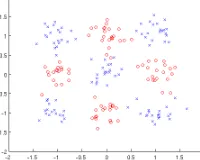
σ2= 0.04 andI is the identity matrix. The points generated for the training set are shown in Figure 8.
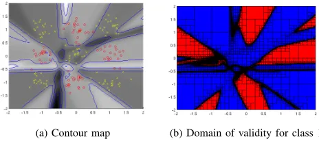
For this problem we trained a number of different feed-forward neural network varying the number of nodes in the hidden layer in order to examine how the validity domain of the neural network changes with the number of hidden nodes. Results are displayed in Figures 9, 10, 11 and 12 for 6, 8, 10 and 15 nodes in the hidden layer, respectively.
By simple observation of the results for this problem
Fig. 8:The artificial problem with 2 classes and 9 groups
[image:6.612.394.494.569.649.2] [image:6.612.124.230.615.704.2](a) Contour map (b) Domain of validity for class 1
Fig. 9:The 2 classes - 9 groups problem for a 2-6-1 network
[image:7.612.59.293.252.354.2](a) Contour map (b) Domain of validity for class 1
Fig. 10:The 2 classes - 9 groups problem for a 2-8-1 network
(a) Contour map (b) Domain of validity for class 1
Fig. 11:The 2 classes - 9 groups problem for a 2-10-1 network
(a) Contour map (b) Domain of validity for class 1
Fig. 12:The 2 classes - 9 groups problem for a 2-15-1 network
network with 8 hidden nodes is the bigger among all other areas reported for the experiment. Though this finding is an empirical one, it coincides with the well known theoretical argument that the mapping capability of a neural network depends on the number of the hidden layer nodes. Moreover, it is surprising to see that a theoretical issue is experimentally verified here. This issue is that, the networks with sufficiently few hidden nodes provide the best performance in terms of generalization. Indeed, the area covered by the 2-8-1 network accounts for 5.94square units, while the 2-10-1 network does
4.41and the 2-15-1 network4.55of the total16square units of the input space. Needless to say that the 2-6-1 network has serous difficulties in approximating the classification function and it gives only 3.30 units. We believe that this provides a strong evidence that by using the proposed inversion technique, it is possible to evaluate the effectiveness of a neural network in terms of approximating the classification function.
4) The Fisher-Iris problem: We also carried out some indicative simulations with the Fisher-Iris problem. Given that the input dimension of this problem is 4 instead of trying to visualize the results of the neural network inversion we performed some checking regarding the findings of the previ-ous paragraph, that is, the area of the domain of validity with respect to the number of hidden layer nodes. The experiments were carried out with two networks with one hidden layer having 2 and 5 nodes, respectively. The nodes in the hidden layer use the hyperbolic tangent activation function while the output ones are pure linear. For example, we have that the area of the domain of validity detected for class 1 (Setosa) for these two networks are,2.3552for the 4-2-3 network and2.0328for the 4-5-3 network. These numbers support the results derived by the previous experiment.
IV. DISCUSSION
A. Interpreting the area of the domain of validity
Suppose that we have a multi-layer perceptron (MLP) with one hidden layer having h nodes which is trained on a general M-class classification problem. The MLP is given a sample data set D = (X, Y) of P objects defined by the n-dimensional patterns x1, x2, . . . , xP. In addition, let C1, C2, . . . , CM denote the M classes of the classification
problem. As we have seen, the inversion of the trained MLP, using SIVIA, results in partitioning the pattern space in a number of disjoint regions. For each specific class this network inversion reveals the part of the input space which is mapped inside those interval of the network outputs’ range which correspond to some specific class of the input patterns.
More specifically, for each class Cj,1 6 j 6 M,
network inversion results in defining a set of Nj boxes {B1, B2, . . . , BNj}, with Bk ∈ R
n for 1
6k 6Nj, whose
union XIn,j = S Nj
k=1Bk encloses the part of the pattern
space containing all the patterns that the network maps to class Cj. If VBk denotes the volume of the box Bk then
the total volume of the input area for class Cj is given by VCj =
PNj
k=1VBk. Any pattern not belonging to class Cj
but found inside the area enclosed byXIn,j is a misclassified
pattern and so an elementary volume Velem corresponding to
this pattern needs to be subtracted from VCj. The resulting
volume, VCj, provides a quantitative estimation of the part of
[image:7.612.59.294.423.526.2] [image:7.612.59.291.595.698.2]computed by the MLP.
In the context of our approach, neural network inversion establishes for each class Cj a mapping between a specific
area of the input space and the MLP output encoding the membership to classCj for any pattern from this specific area.
Hence, we expect that the estimation of Bayesian probabilities defined by the network outputs are mapped via network inversion to respective measures (Bayesian probabilities) in the input space. We consider this statement being true if we take into account the volumes in the input space, as defined above, and define the following quantities
VC1 Vtotal
, VC2 Vtotal
, . . . , VCM
Vtotal
,Vmissd Vtotal
,Vuncrt Vtotal
. (5)
All these ratios give positive real number which sum up to 1. So they seem to be a sort of probabilities which are related to the network output values. Such an empirical conclusion is a conjecture that needs to be further studied especially in a context such as the one presented by Richard and Lippmann [22]. We expect this study to shed light in the reliability aspects of neural network generalization.
B. Interpretation in terms of best fitting model
It is common knowledge in the neural network research area that different number of nodes in the hidden layer of an MLP define different network architectures which in their turn define different models for the underlying process. It has also been verified, by our experiments, that for the same input data set D = (X, Y) different models provides a different classification function with different results. Suppose that a number of different modelsH1,H2, . . . ,HLare available after
training of the respective network architectures for the problem at hand. Moreover, for each one of these models, say Hl,
network inversion computes a partition of the input space which is specific for this model.
When a number of different models approximate a problem the question posed is which one of these models fits better the sample data D available for the problem. In terms of a Bayesian decision framework, if one requires to assess the best model for the problem one needs to estimate the plausibility of each one of the models H1,H2, . . . ,HL. So,
using Bayesian inference to evaluate model plausibility given the dataD, we first need to compute the posterior probability
P(Hl|D)for each model and the perform model comparison. In consequence, for each modelHlone needs to consider that
P(Hl|D)∝P(D|Hl)P(Hl). (6)
In order to compute the left hand side of the previous relation one needs to compute the likelihood of the model P(D|Hl)
and the prior P(Hl). For some model Hl a priori we have
no reason to believe that this model fits better the data than the other models and so the prior probability P(Hl) is the
same for all available models. Hence, in order to consider some model Hl more plausible than the others we need to compute the posterior probability P(D|Hl). At this point, if the previous analysis of the previous subsection is true we may use the quantityVclassd/Vtotal to approximateP(D|Hl).
C. Other issues
Other important issues regarding the proposed method are those concerning performance related to the application of SIVIA. The experimental verification of the method, presented here, concerns low dimension problems and small sized neural networks. Further experiments are needed on problems with higher input dimension and medium sized network. This is mandatory in order to verify that no overestimation effects are produced when performing interval computations with neural networks in higher dimension problems.
Inverting a neural network and estimating its domain of validity with SIVIA is an exhaustive research process of the input space. Hence, performance of the method is exponential with the number and the domain of the inputs. However, given that inversion is typically done off-line, after a network has been trained, it is legitimate to consider that applying SIVIA is affordable when used off-line.
V. CONCLUSION
In this paper we presented a new approach to perform accurate estimation of the domain of validity of feed-forward neural networks. The approach relies exclusively on IA con-cepts making use of SIVIA a method performing set inversion via interval analysis. SIVIA has been successfully applied to problems where nonlinear analysis is involved. Hence, defining the domain of validity of a neural network is considered to be a nonlinear parameter estimation problem. The method was experimentally tested on a number of problems and the results obtained in terms of detecting the domains of validity proved to be very promising for obtaining reliable conclusions on aspects of the neural network such as its ability to generalize well and its ability to be explicative. Compared to contour maps the proposed method has the advantage to provide quantitative information on the part of the input space covered by the domain of validity.
The domain of validity may be used to indicate the part of the input area where the network is stable in terms of classification. Another tangible result concerns the possibility to define rules describing in symbolic terms the classification function. In the paper we discussed a number of issues that seem to characterize the generalization ability of the neural network both in terms of estimating a probability of correct classification as well as in terms of the effectiveness of a network architecture to correctly map the input space. We believe that, these issues constitute interesting questions for carrying on the research initiated in this paper.
REFERENCES
[1] L. Jaulin and E. Walter, “Set Inversion Via Interval Analysis for nonlinear bounded-error estimation,” Automatica, vol. 29, no. 4, pp. 1053–1064, 1993.
[2] P. Courrieu, “Three algorithms for estimating the domain of validity of feedforward neural networks,” Neural Networks, vol. 7, no. 1, pp. 169–174, 1994.
[3] M. Pelillo, “A relaxation algorithm for estimating the domain of validity of feedforward neural networks,” Neural Processing Letters, vol. 3, no. 3, pp. 113–121, 1996.
[5] R. J. Williams, “Inverting a connectionist network mapping by back-propagation of error,” in Proc. 8th Annu. Conf. Cognitive Sci. Soc.
Hillsdale, NJ: Lawrence Erlbaum, 1986, pp. 859–865.
[6] J. Kindermann and A. Linden, “Inversion of neural networks by gradient descent,”Parallel Computing, vol. 14, no. 3, pp. 277 – 286, 1990. [7] R. Eberhart and R. Dobbins, “Designing neural network explanation
facilities using genetic algorithms,” in Neural Networks, 1991. 1991 IEEE International Joint Conference on, vol. 2, Nov 1991, pp. 1758– 1763.
[8] R. Reed and R. Marks, “An evolutionary algorithm for function in-version and boundary marking,” inEvolutionary Computation, 1995., IEEE International Conference on, vol. 2, Nov 1995, pp. 794–797. [9] M. I. Jordan and D. E. Rumelhart, “Forward models: Supervised
learning with a distal teacher,” Cognitive Science, vol. 16, no. 3, pp. 307–354, 1992.
[10] B.-L. Lu, H. Kita, and Y. Nishikawa, “Inverting feedforward neural networks using linear and nonlinear programming,”Neural Networks, IEEE Transactions on, vol. 10, no. 6, pp. 1271–1290, Nov 1999. [11] E. W. Saad and D. C. W. II, “Neural network explanation using
inversion,”Neural Networks, vol. 20, no. 1, pp. 78–93, 2007. [12] S. B. Thrun, “Extracting Provably Correct Rules from Artificial Neural
Networks,” Institut fur Informatik III, Bonn, Germany, Technical Report IAI–TR–93–5, 1993.
[13] R. J. H. Filer and J. Austin, “Feedforward Rule Extraction from Neural Networks by Interval Analysis,” Department of Computer Science, The University of York. [Online]. Available: http://ofuturescholar.com/paperpage?docid=487066
[14] C. Hern´andez-Espinosa, M. Fern´andez-Redondo, and M. Ortiz-G´omez, “Inversion of a Neural Network via Interval Arithmetic for Rule Extraction,” in Artificial Neural Networks and Neural Information Processing ICANN/ICONIP 2003, ser. Lecture Notes in Computer Science, O. Kaynak, E. Alpaydin, E. Oja, and L. Xu, Eds. Springer Berlin Heidelberg, 2003, vol. 2714, pp. 670–677.
[15] K. Kwon, H. Ishibuchi, and H. Tanaka, “Nonlinear Mapping of Interval Vectors by Neural Networks,” inNeural Networks, 1993. IJCNN ’93-Nagoya. Proceedings of 1993 International Joint Conference on, vol. 1, Oct 1993, pp. 758–761.
[16] G. Alefeld and G. Mayer, “Interval Analysis: Theory and Applications,”
Journal of Computational and Applied Mathematics, vol. 121, pp. 421– 464, 2000.
[17] L. Jaulin, M. Kieffer, O. Didrit, and E. Walter,Applied Interval Analysis. with Examples in Parameter and State Estimation, Robust Control and Robotics. London: Springer–Verlag, 2001.
[18] L. Jaulin, “Technical Communique: Interval Constraint Propagation with Application to Bounded-error Estimation,” Automatica, vol. 36, no. 10, pp. 1547–1552, Oct 2000.
[19] S. Tornil-Sin, V. Puig, and T. Escobet, “Set Computations with Sub-pavings in MATLAB: The SCS Toolbox,” inComputer-Aided Control System Design (CACSD), 2010 IEEE International Symposium on, Sept 2010, pp. 1403–1408.
[20] S. M. Rump, “INTLAB – INTerval LABoratory,” inDevelopments in Reliable Computing, T. Csendes, Ed. Dordrecht, Netherlands: Kluwer Academic, 1999, pp. 77–104.
[21] S. Theodoridis, A. Pikrakis, K. Koutroumbas, and D. Kavouras, Intro-duction to Pattern Recognition: A MATLAB Approach. Burlington, MA 01803, USA: Academic Press, 2010.
![Fig. 1: A function f, an inclusion function [f] and the images of [x]](https://thumb-us.123doks.com/thumbv2/123dok_us/8867513.940657/4.612.326.553.60.192/fig-function-f-inclusion-function-f-images-x.webp)