BIROn - Birkbeck Institutional Research Online
Briant, Rebecca and Cohen, K. and Cordier, S. and Demoulin, A. and
Macklin, M. and Mather, A. and Rixhon, G. and Veldkamp, A. and Wainwright,
J. and Whittaker, A. and Wittmann-Oelze, H. (2018) Applying Pattern
Oriented Sampling in current fieldwork practice to enable more effective
model evaluation in fluvial landscape evolution research.
Earth Surface
Processes and Landforms 43 (4), pp. 2964-6980. ISSN 0197-9337.
Downloaded from:
Usage Guidelines:
Please refer to usage guidelines at or alternatively
1
Applying Pattern Oriented Sampling in current fieldwork practice to enable more effective model
1
evaluation in fluvial landscape evolution research
2
*Briant, R.M., Cohen, K.M., Cordier, S.Demoulin, A., Macklin, M.G., Mather, A.E., Rixhon, G.,
3
Veldkamp, A., Wainwright, J., Whittaker, A., Wittmann, H. 4
Studies using Landscape Evolution Models (LEMs) on real-world catchments are becoming 5
increasingly common. Evaluating their reliability requires us to bring together field and model data. 6
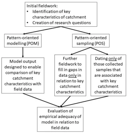
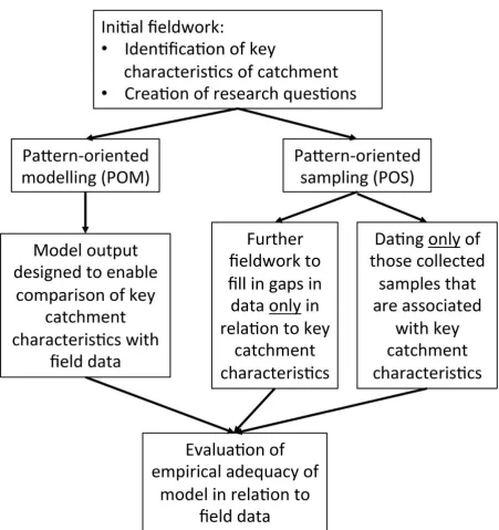
We argue that these are best synchronised by complementing the Pattern Oriented Modelling 7
(POM) approach of most fluvial LEMs with Pattern Oriented Sampling (POS) fieldwork approaches 8
(Figure 1). 9
[image:2.595.74.483.257.694.2]10
Figure 1 – Flow chart for applying Pattern Oriented Modelling (POM) and Pattern Oriented
11
Sampling (POS) within a join field-model investigation of a specific catchment.
12
2
Applying Pattern Oriented Sampling in current fieldwork practice to enable more effective model
14
evaluation in fluvial landscape evolution research
15
16
1Briant, R.M., 2Cohen, K.M., 3Cordier, S. 4Demoulin, A., 5,6Macklin, M.G., 7Mather, A.E., 8Rixhon, G.,
17
9Veldkamp, A., 10Wainwright, J., 11Whittaker, A., 12Wittmann, H.
18
Lead author email address: [email protected] 19
1Department of Geography, Environment and Development Studies, Birkbeck, University of London,
20
Malet Street, London, WC1E 7HX, U.K. 21
2Department of Physical Geography, Utrecht University, PO box 80.115, 3508 TC Utrecht, The
22
Netherlands 23
3Département de Géographie et UMR 8591 CNRS- Université Paris 1-Université Paris Est Créteil,
24
Créteil Cedex, France 25
4Department of Physical Geography and Quaternary, University of Liège, Sart Tilman, B11 - 4000
26
Liège, Belgium 27
5School of Geography, University of Lincoln, Brayford Pool, Lincoln, Lincolnshire, LN6 7TS, U.K.
28
6Institute Agriculture and Environment, College of Sciences, Massey University, Private Bag 11 222,
29
Palmerston North 4442, New Zealand 30
7School of Geography, Earth and Environmental Sciences, University of Plymouth, Drake Circus,
31
Plymouth, Devon, PL4 8AA, UK 32
8Laboratoire Image, Ville, Environnement (LIVE), UMR 7362 - CNRS, University of
Strasbourg-33
ENGEES, 3 rue de l’Argonne, 67083 Strasbourg, France 34
9ITC, Faculty of Geo-Information Science and Earth Observation of the University of Twente, PO Box
35
217, 7500 AE Enschede, The Netherlands 36
10Durham University, Department of Geography, Science Laboratories, South Road, Durham, DH1
37
3LE, UK 38
11Department of Earth Science and Engineering, Imperial College London, South Kensington Campus,
39
London SW7 2AZ, UK 40
12Helmholtz Centre Potsdam, GFZ German Research Centre for Geosciences, Telegrafenberg, 14473
41
Potsdam, Germany 42
3
Note: Yellow highlighted text is completely new (other new text has been added but is less
44
substantial), green highlighted text is substantially reworked
45
Abstract
46
Field geologists and geomorphologists are increasingly looking to numerical modelling to understand 47
landscape change over time, particularly in river catchments. The application of Landscape Evolution 48
Models (LEMs) started with abstract research questions in synthetic landscapes. Now, however, 49
studies using LEMs on real-world catchments are becoming increasingly common. This development 50
has philosophical implications for model specification and evaluation using geological and 51
geomorphological data, besides practical implications for fieldwork targets and strategy. The type of 52
data produced to drive and constrain LEM simulations has very little in common with that used to 53
calibrate and validate models operating over shorter timescales, making a new approach necessary. 54
Here we argue that catchment fieldwork and LEM studies are best synchronised by complementing 55
the Pattern Oriented Modelling (POM) approach of most fluvial LEMs with Pattern Oriented 56
Sampling (POS) fieldwork approaches. POS can embrace a wide range of field data types, without 57
overly increasing the burden of data collection. In our approach, both POM output and POS field 58
data for a specific catchment are used to quantify key characteristics of a catchment. These are then 59
compared to provide an evaluation of the performance of the model. Early identification of these 60
key characteristics should be undertaken to drive focused POS data collection and POM model 61
specification. Once models are evaluated using this POM / POS approach, conclusions drawn from 62
LEM studies can be used with greater confidence to improve understanding of landscape change. 63
Keywords
64
Landscape evolution modelling, Pattern Oriented Sampling, catchments, fluvial systems, geological 65
field data 66
Introduction
67
Traditionally landscape evolution models have been heuristic models based on elaborate fieldwork 68
campaigns encompassing mapping and description of relevant landforms and deposits (e.g. Davis, 69
1922). The interpretation of the collected data on topography, bedrock and sediments of hillslopes 70
and valleys yielded chronological narratives centred around the available evidence (e.g. Maddy, 71
1997; Gibbard and Lewin, 2002). These narratives often used simple linear cause and effect 72
reasoning tailored to specific locations and prone to disciplinary biases. A danger with such models is 73
that they may then be applied as universal conceptual models in other locations where key 74
processes differ. The growing awareness that Earth is a coupled system with many global dynamics 75
caused researchers to incorporate known global oscillations such as in tectonics (e.g. Milliman and 76
Syvitski, 1992), climate (Vandenberghe, 2008; Bridgland and Westaway, 2008), base-level (Talling, 77
1998) and glaciation (e.g. Cordier et al., 2017) into their heuristic models. However, since it has 78
become more widely known that earth surface processes have non-linear complex dynamics it has 79
also become clear that simple linear cause and effect stories do not accurately capture all real world 80
4 records (e.g. Schumm, 1973; Vandenberghe, 1993; Blum and Törnqvist, 2000; Jerolmack and Paola, 82
2010). 83
Alongside this, the use of numerical landscape evolution models has accelerated. Since the early 84
1990s (see review by Veldkamp et al., 2017) these have developed into tools used to undertake 85
theoretical experiments about the complexity of earth surface processes, although under controlled 86
and strongly simplified conditions. Because they were invented to explore theoretical questions 87
about past forcings within landscapes, these Landscape Evolution Models (LEMs) are significantly 88
different from other types of models that simulate and forecast processes operating at present. Not 89
least, their relation to field data is only now being assessed in detail, since initial studies frequently 90
used synthetic landscapes (e.g. Whipple and Tucker, 1999; Wainwright, 2006). 91
There are five main groups of numerical models that deal with the earth surface processes: 92
climatological, hydrological, ecological, hydraulic-morphodynamic and LEMs. Landscape evolution 93
models are distinctive because they combine elements of the other four, frequently enabling all 94
domains to change during a model run rather than modelling one and specifying others as input 95
parameters. In doing this, they focus on long-term geomorphology – both the form of the landscape 96
and the processes operating within it (e.g. Temme et al., 2017). Whilst some geomorphological 97
features form quickly and can be monitored and modelled in parallel to hydraulic measurement and 98
modelling (e.g. Camporeale et al. 2007), evolution of a full geomorphological landscape takes several 99
orders of magnitude longer than human monitoring. The record that remains is therefore scattered 100
and incomplete. As such, the cases being modelled are inherently more intractable. This is not only 101
because process observations, even ‘long-term’ ones, rarely scale to the geological timescales under 102
study (parameters of the LEM can account partially for this, see Veldkamp et al., 2017), but even 103
more so because the initial conditions required for the LEM cannot be specified simply from modern 104
datasets, even though LEMs are notoriously sensitive to the specification of initial conditions. LEMs 105
share these characteristics of underdetermination with geodynamic models (e.g. Garcia-Castellanos 106
et al., 2003), where key processes and features being modelled occur beneath the land surface and 107
therefore very few initial conditions or processes can be directly measured. In addition, because 108
more features of the landscape are allowed to change in a LEM than in the other types of earth 109
surface models (Mulligan and Wainwright, 2004), they require a different approach, analogous to 110
the difference between modern climate and palaeoclimate modelling (Masson-Delmotte et al., 111
2013). 112
Many non-LEM models seek numerical prediction (e.g. Oreskes et al., 1994), or at least robust 113
projection of potential scenarios into the future, based on detailed comparison to a short time 114
period of ‘the past’. This is because many of these other types of model (climate, hydrology and 115
ecology) are used as a basis for future policy planning. Thus such models seek to replicate ‘reality’ 116
more and more closely, as can be seen in the explosion of complexity in General Circulation Models 117
from the 1970s to the present day (e.g. Taylor et al., 2012). This replication of reality is seen in 118
increased inclusion of processes, but also in calibration, where parameters are tuned to known field 119
observations to produce outputs that are as close to measured reality as possible. Once these non 120
LEM models are validated using a different subset of past data, numerical prediction commences 121
5 In contrast, landscape evolution modelling does not aim for exact replication of present day
123
landscapes, although a measure of this is required to evaluate the usefulness of the model. Rather, 124
the focus in most location-specific LEM studies is on narrowing down the range of processes likely to 125
have been operating in a particular catchment in the geological past. For this reason calibration as 126
defined above is rarely undertaken because numerical predictions are not required. This is not least 127
because the difference between what is being modelled and what can be measured is greater than 128
in (for example) hydrological models. For example in relation to temporal scale, the length of time 129
being modelled means that the time steps necessarily used have little physical meaning (e.g. 130
Codilean et al., 2006). Furthermore, some sets of parameter values that seem to fit the data well 131
lack physical plausibility, questioning the value of applying calibration to LEMs, e.g. van der Beek and 132
Bishop (2003). In addition, because of these longer timescales many properties are required to 133
change in landscape evolution modelling that are frequently kept constant in hydrological models. 134
These changing elements propagate impacts and uncertainties in space and time and the 135
introduction of parameterisation arguably increases these uncertainties by introducing an additional 136
level of uncertainty (Mulligan and Wainwright, 2004). Therefore, with landscape evolution models, 137
the aim is not for more and greater complexity over time, but to constrain uncertainties as much as 138
possible. Because the research questions being addressed usually involve explanation, the goal is to 139
generate a plausible narrative based on the (frequently sparse) data available – just as in a forensic 140
investigation - and not to achieve a numerical outcome that is ‘correct’ although some measure of 141
the accuracy of approximation of the landscape to the present day is of course required for 142
evaluation. Key research questions are likely to be framed as (e.g. Larsen et al., 2014): which are the 143
most likely modes of formation for the landscape observed? What types or scales of tectonic activity 144
are most likely to produce the landforms observed? What characteristics of a catchment enable a 145
climate signal to be successfully transferred into a sedimentary record? As noted by Temme et al. 146
(2017), the more complete the data available, the more catchment-specific the questions that can 147
be addressed. Often, however, complete landscape and process reconstruction is not possible. 148
Providing evidence to choose between competing hypotheses is more common (e.g. Viveen et al., 149
2014). 150
In order to generate a plausible narrative of landscape change, complexity is often actively reduced 151
(e.g. Wainwright and Mulligan, 2005). Processes and parameters are only included in an LEM if there 152
is evidence that they are likely to be relevant for explanation. This approach of ‘insightful 153
simplification’ or ‘reduced complexity modelling’, does seek to explain what has happened in a 154
specific place, as in the traditional heuristic model, but also to more broadly understand the known 155
global driving factors within fluvial landscapes (Veldkamp and Tebbens, 2001), and to create 156
generalizable statements about the development of large-scale geomorphological features. A 157
further advantage of seeking simplification with complex feedbacks is that it allows emergent 158
behaviour. In this case, a relatively simple set of factors is modelled, but can lead to apparently 159
complex behaviour (e.g. Schoorl et al, 2014). 160
The above listed differences in approach between LEMs and other groups of earth surface models, 161
encompass both philosophical issues in modelling and the relationship between models and field 162
observations. This paper, whilst exploring the philosophical issues, seeks mainly to address the issue 163
of field-model data comparison to evaluate LEM output created using this insightful simplification 164
approach. It is aimed predominantly at field scientists, enabling them to apply the multiplicity of 165
6 evolution model output and geological field data. In this paper, we argue that field data collection 167
strategies and LEM studies are best brought together by deploying Pattern Oriented Sampling (POS) 168
approaches when collecting field data. In this way, key characteristics of a real-world catchment are 169
identified (e.g. sediment distribution, thalweg gradient, floodplain width) in both past timeslices and 170
in the end situation and used to compare with the same characteristics generated from LEM output. 171
The Pattern Oriented Sampling approach that we advocate serves to collect field data that is more 172
useful for comparison with model output. Improving our ability to evaluate model output will then 173
allow us to use LEMs to narrow the range of plausible narratives that explain the field data observed. 174
In this way, we will be able to generate more robust generalisations than either those based on 175
location-specific heuristic / conceptual models (e.g. Bridgland and Westaway, 2008) or those using 176
synthetic landscapes (e.g. Whipple and Tucker, 1999). Whilst there are philosophical difficulties with 177
strict validation of models of inherently open natural systems (Oreskes et al., 1994), evaluation of 178
such modelling work against relevant field datasets is still crucial to determine at least the empirical 179
adequacy of each model (e.g. Coulthard et al., 2005; Van De Wiel et al., 2011; Veldkamp et al., 180
2016). 181
It is our contention that the nature and scarcity of much geological field data, which are typically not 182
randomly generated, preserved or sampled, makes this a different and more intractable process for 183
LEMs than for example hydrological modelling. Whilst it is true that all earth surface process models 184
face problems of comparison with a limited set of field observations, this has mostly to do with bias 185
and gaps in data collection. Because of the time scales involved, field data for comparison with LEM 186
outputs have the additional problem that the geological and geomorphological records (deposits and 187
erosional surfaces alike) are in large part removed and reworked by processes operating since they 188
were first generated. Furthermore, most data are proxies for actual land surface characteristics that 189
may or may not have analogues in the present day. Nonetheless, we argue that our Pattern Oriented 190
sampling can significantly improve the suitability of geological field data selected for model 191
evaluation. 192
We focus on fluvial landscape evolution in this paper, but some of the general points raised are also 193
relevant for modelling landscape evolution in other process domains. We will first discuss key 194
philosophical considerations in applying field data to LEM evaluation. This is followed by advocating 195
the use of a catchment wide Pattern Oriented Sampling (POS) approach to support fieldwork 196
inventories, showing how such an approach might apply in different settings. This is a companion 197
paper to Temme et al. (2017), which addresses a similar question from a numerical modelling 198
perspective. Both papers arise from the newly created FACSIMILE (Field And Computer SIMulation In 199
Landscape Evolution) network, which brings together European modellers and field-based 200
geoscientists investigating landscape evolution at various scales with both tectonic and climatic 201
drivers. This Pattern Oriented Sampling approach allows a more direct comparison with the Pattern 202
Oriented Modelling approaches of numerical fluvial landscape evolution models at multiple spatial 203
and temporal scales. 204
Philosophical considerations in applying field data to LEM evaluation
205
Calibration and parameterisation
7 Parameterisation is the inclusion of the most relevant processes for the questions being asked in a 207
particular modelling study. Calibration is setting these parameters to meaningful values for the 208
specific location being modelled. When LEMs are used for studies that fall within the historic time 209
period, then field data is sometimes used for model calibration – i.e. to inform and empirically adjust 210
the parameterisation of the model (see for example Veldkamp et al., 2016). This process can also 211
enable useful learning about model function (Temme et al., 2017). We would argue however that 212
this full calibration is neither common nor useful for geological time-scale LEM studies. This is 213
despite the fact that landscape evolution models contain multiple spatially-varying parameters that 214
may have only a poor relation to field measurements (containing unmeasurable units such as 215
erodibility) and would thus traditionally be targeted for significant calibration. This is because the 216
aim of many landscape evolution models is to explore process outcomes, rather than to closely 217
mimic field results or provide numerical prediction. As stated by Temme et al (2017, p. 28) 218
‘calibration typically distinguishes studies where models support field reconstruction from studies 219
where models are used in a more exploratory manner to ask ‘what-if’ questions about landscape 220
development.’ Whilst it could be argued that prediction could also be used as a term to refer to the 221
interpolation of data spatially or temporally within the modelling process to estimate a value that 222
has not been or cannot be measured this is not the definition of prediction that we are using here. 223
We argue that such temporal interpolation is merely an extension of the process of exploring 224
different pathways of landscape development. Because the models are not required for prediction, 225
extensive calibration of parameters to a specific geomorphological setting is of less value, and 226
indeed might ‘tend to remove the physical basis of a model’ (Mulligan and Wainwright, 2004, p. 55), 227
for example when parameters are given values that do not make physical sense. It is this physical 228
basis that enables investigation of process outcomes and we would therefore argue needs to be 229
retained. 230
This retention of basic physics is particularly important because rules drawn from short-term process 231
observations do not scale up easily to longer timescales. One reason for this is that magnitude-232
frequency distributions of the parameterised events driving the process may have been different in 233
the past, particularly when there is no suitable present day analogue. For example, whilst it is clear 234
that periglacial processes have played an important role in fluvial activity and geomorphological 235
change over Pleistocene timescales across Eurasia and North America (e.g. Vandenberghe, 2008), 236
and we understand the links between annual temperature cycle variations and periglacial processes 237
in the modern circum-arctic very well, yet we have no understanding of how such annual freeze-238
thaw processes differ when occurring in mid-latitude rather than Arctic regions (e.g. Murton and 239
Kolstrup, 2003). 240
In the situation where one is forced to parameterise processes for settings lacking an analogue 241
situation, which is very common when using LEMs, we argue that the researcher should avoid a full 242
calibration of said parameters because it introduces greater certainty into the modelling than there 243
is in the real world. Instead, a wider range of process pathways need to be explored in the LEM than 244
possible using the subset of partial analogue settings for which calibration data would be available. 245
Indeed, not calibrating parameters allows the investigation of process outcomes to also include 246
experiments in which different values of these parameters are investigated, rather than a narrower 247
range of experiments in which they have been ‘optimised’ in advance of the reported modelling 248
8 other parameters in that LEM were varied in series of experimental scenarios. Similarly, a restricted 250
range of values can be set for a parameter on the basis of field data without specifying a single value 251
through a traditional parameterisation process (e.g. erosion rates estimated between two dated lava 252
flow events – van Gorp et al., 2015). 253
Validation versus evaluation
254
A second issue to be considered is that of validation. As Oreskes et al. (1994) state, this is intimately 255
linked with the process of calibration, which we discuss above. Strict validation uses a separate 256
dataset to that used for initial model specification and parameter calibration. However, over 257
geological time scales, information relating to each parameter is often too sparse to afford the 258
luxury of splitting a dataset into calibration and validation subsets. Indeed, it is usually the case that 259
almost all the information available is used to specify initial conditions and narrow down the range 260
of parameters used in model runs. Because of this, the only way in which a separate dataset can be 261
generated for validation is by systematically leaving out part of the collected data and using only this 262
data to compare with the key patterns emerging from model outputs in a form of quasi-validation 263
(e.g. Veldkamp et al., 2016). Whilst not strictly independent, this type of quasi-validation is often 264
sufficient to indicate if the LEM simulation is in the correct range of process rates and timing. As 265
discussed in more detail below, and in Table 2, some quantification of the success of this evaluation 266
/ quasi-validation is useful if possible, even though the use of R2 values to score performance is
267
usually inappropriate. 268
Equifinality
269
Thirdly, equifinality is worth discussing because most LEM modelling of river catchments runs 270
forward from some initial situation and ends in a simulation of ‘the present’. The model output for 271
the present is the simplest to both evaluate (comparing modelled and field data) and analyse 272
(tracing development through time) for explanatory understanding of landscape evolution and the 273
geological / geomorphological record preserved from it. This approach is of course sensitive for 274
equifinality, considering that the generated end state in simulations can be reached in many ways 275
starting from different initial conditions and physical assumptions, whereas in the real world it was 276
just one path. Equifinality is well known to play an important role in fluvial records and their 277
modelling by dedicated LEMs (Beven, 1996; Nicholas and Quine, 2010; Veldkamp et al., 2017). Such 278
modelling is therefore often coupled with the use of multiple model runs to capture the range of 279
statistical variability between different runs with either fixed or varying parameters. The narrative 280
favoured for explanation is then adopted from the modelled scenario with the best fit to the present 281
day (e.g. Bovy et al., 2016). Where only one scenario fits the geological data available for evaluation, 282
equifinality is avoided. However, we argue here that whilst a single modelled scenario can 283
sometimes be chosen, this is not always helpful in advancing understanding. Indeed, where more 284
than one scenario fits well to the present day, we argue that this should be embraced as defining an 285
envelope of possible explanations, narrowing down our understanding of the processes that could 286
produce such a suite of features without suggesting an unrealistic level of certainty about which 287
landscape history has taken place. If a single solution is still desired, a valuable way of dealing with 288
equifinality in such settings is to gradually work through multiple competing hypotheses. This has 289
9 conceptual models and has recently been adopted by some ecologists, e.g. Johnson and Omland 291
(2004). It has been shown to be particularly useful in evolutionary biology, a field that bears 292
remarkable similarity to landscape evolution modelling, given the long time-scales involved, lack of 293
data from many time periods other than the present, and the possibility of equifinality e.g. Lytle 294
(2002). A more recent example of this in landscape evolution is the use of field data alone to 295
determine the relative importance of seepage compared to runoff in canyon formation (Lamb et al., 296
2006). The two stage LEM strategy of Braun and van der Beek (2004) also demonstrates the gradual 297
investigation of different hypotheses, with a second stage adding in modelling of the lithosphere to 298
enable differentiation between two similar outputs based on different synthetic initial topographies. 299
Initial conditions
300
Fourthly, the influence of initial conditions should be considered. When the modelling exercise is 301
carried out in a real-world (rather than synthetic) landscape, specifications of the initial digital 302
elevation model (DEM - resolution, x, y and z accuracy) and surface characteristics (sediment 303
thickness, grain size distribution and erodibility) are particularly important. Whilst all models that 304
forward-simulate open systems require specification of initial conditions (e.g. snow cover or soil 305
moisture in hydrological modelling), specifying initial conditions for geological timescales is 306
particularly problematic because of the scale of difference from modern conditions. This is discussed 307
above in relation to calibration and does not apply to other earth surface model types. This scale of 308
difference is important because uncertainty propagation through the modelling process to output 309
DEMs may be significant, and as discussed above equifinality can also play a role in such outcomes. 310
For example, if starting topography ‘contains the common processing artefact of steps near contour 311
lines, these steps will tend to become areas of strong localised erosion and deposition that can 312
obscure the larger patterns’ (Tucker, 2009, p. 1454). There are two approaches to specifying the 313
initial DEM. The first is to use the modern land surface. This is only possible if change over time is 314
minimal and topographic data are not used to evaluate model outputs. It has the advantage that the 315
uncertainty relating to spatial resolution and associated interpolation is low (e.g. as investigated by 316
Parsons et al., 1997, for hydrological modelling). However, the longer the time period to be 317
modelled, the greater the error associated with using such a surface, especially in models where 318
sensitivity to initial conditions is a significant feature. For example, use of a modern DEM is not 319
appropriate where sediments known to be deposited during the time period modelled are present 320
below the modern land surface or when studying a tectonically triggered episode of deep valley 321
incision (e.g. van de Wiel et al, 2011). 322
Defining an alternative initial DEM or ‘palaeoDEM’ requires expert judgment based on field 323
experience that is not easily harvested from literature. For example, when incision over time is the 324
main focus, it may be possible to determine surfaces within the landscape from which incision is 325
likely to have started using modern land-surface DEMs as a starting point, such as relict long profiles 326
(e.g. Beckers et al., 2015) or reliably reconstructed and dated palaeosurfaces (e.g. Fuchs et al., 2012). 327
A number of numerical approaches can be adopted here, as outlined by Demoulin et al. (2017). 328
Expert judgment can also suggest palaeosurfaces based on sedimentological investigations. For 329
example, erosional contacts may suggest initial surfaces lay higher prior to a period of erosion, but 330
gradational contacts that initial surfaces were close to the base of the sequence. Such delineation is 331
10 a typical main channel and thus truly deviate from modern surface conditions (e.g. Boenigk &
333
Frechen, 2006). The disadvantage of using a reconstructed palaeosurface as an initial DEM is that 334
they are ‘typically of very coarse spatial resolution, smoothed and subject to considerable 335
uncertainty’ (van de Wiel et al., 2011, p. 179). A useful recent development is the application of 336
geospatial interpolation to refine field derived terrace data sets for palaeosurface reconstructions 337
(Geach et al., 2014; van Gorp et al., 2015). This approach can improve the resolution of the initial 338
DEM and thus the quality of the end results but cannot resolve the fundamental problem of 339
reconstructing the unknown. 340
The specification of an initial DEM is particularly important for LEMs because the scale of the 341
difference between modern and past landscapes is likely to be large with different processes 342
contributing to their formation (Temme & Veldkamp, 2009). However, it should also be undertaken 343
with caution because of this. We therefore propose that future studies should give more thought to 344
initial land surfaces and their conditions whilst field investigation is being undertaken rather than at 345
a later date. If field investigation suggests that the modern land surface is the most appropriate 346
initial DEM to use then the field worker should liaise closely with the modeller to get the highest 347
possible resolution data. This will be only over very short time periods of a century or less where the 348
scale of change is sufficiently small that the additional error gained from using a non-modern initial 349
DEM is no longer justifiable (van de Wiel et al., 2011). If, as in most situations, investigation suggests 350
that a palaeosurface / palaeoDEM should be constructed then additional information such as 351
borehole and geophysical data should be collated to maximise the resolution of the surface created 352
and appropriate geospatial interpolation should be applied (Geach et al., 2014; van Gorp et al, 353
2015). Indeed, it might sometimes be wiser to turn the nature of the initial land surface into a 354
research question comparing modern and palaeo-DEMs in different model runs. In this way 355
questions such as the scale of incision or of reworking of sediment within the landscape can be 356
addressed. The multiple working hypotheses approach outlined above and advocated by Temme et 357
al., (2017) can also be used to narrow down the most plausible initial DEM if possible. 358
Catchment choice
359
Finally it is important to consider which catchments are more suitable to study at this moment in 360
time whilst we make the transition in landscape evolution modelling from synthetic to real 361
landscapes. This is pivotal because not all catchments actually record the driving factor of interest 362
(e.g. Fryirs et al., 2007). It has been argued that one should choose catchments that form a ‘natural 363
experiment’ (Tucker, 2009), where only one variable changes over the time period of interest – e.g. 364
modelling channel incision in relation to differential rock uplift in the Mendocino Triple Junction 365
region where other features of the catchments compared are broadly similar (Snyder et al., 2003; 366
Tucker, 2009). However such catchments are rare and we agree with Temme et al. (2017) that we 367
are now at a stage where catchments exhibiting the ‘badass geomorphology’ of Phillips (2015) can 368
be studied, although their complexity needs to be reflected in the research question. We must 369
construct very tightly defined research questions for such catchments, by including or excluding 370
specific external factors from experimental runs (e.g. Coulthard and van de Wiel, 2013). Evidence for 371
catchment response to climate change can be seen by comparing the coincidence of fossil or isotope 372
based climatic reconstructions (e.g. Table 1) with system response (e.g. Lewis et al 2001; Schmitz & 373
11 region is buffered, or even ‘shredded’ with relation to the original signal (Métivier 1999; Castelltort 375
and van den Driessche, 2003; Jerolmack and Paola, 2010; Wittmann et al., 2009; Armitage et al., 376
2013). We can also determine by how much and where it is delayed by intermittent sediment 377
storage related to hill slope – channel (dis)connectivity (Michaelides and Wainwright, 2002; 378
Veldkamp et al., 2015). Evidence for tectonic response can be ascertained by geomorphologic 379
markers distributed within the drainage network, such as slope break knickpoints resulting from the 380
same regional uplift pulse (e.g. Table 1, Beckers et al., 2015). Nonetheless, as noted by Blum et al. 381
(2013), criteria for distinguishing between allogenic and autogenic control in catchments still remain 382
to be tightly defined and it is recognized by Veldkamp et al. (2017) that there is an urgent need for 383
research strategies that allow the separation of intrinsic and extrinsic record signals using combined 384
fieldwork and modelling. 385
It is also worth discussing where the boundaries of the catchment should be drawn. In full source to 386
sink modelling, all four of the following elements would be included: a record from the source, a 387
record from the sink, a model for the source and a model for the sink. When catchments are small, 388
downstream data can comprise field data from alluvial fans, floodplains and lakes containing deltaic 389
and prodeltaic deposits. When a larger catchment is considered, the downstream regions are 390
sedimentary basins with broad valleys and plains (e.g. megafans, distributive fluvial systems – e.g. 391
Davidson et al., 2013; Nichols and Fisher, 2007, Weissman et al, 2015), lakes (e.g. Schillereff et al., 392
2015) and/or delta plains and coastal zones (e.g. basins that form part of continental shelves). Often, 393
as discussed below, downstream data from the sink is not readily available and LEM studies simulate 394
only the source area of the catchment, but this is likely to change as the application of LEMs 395
becomes more widespread. 396
We therefore focus here on the small-medium catchment-scale (c. 10-1000 km long channels) over 397
the later parts of the Quaternary where age control is more robust (c. 500,000 years to present) – 398
there is only so much ‘badass’ behaviour that our LEMs can currently manage. We recognise that for 399
now, this excludes ancient systems where preservation is fragmentary or dating absent or very 400
limited. In such catchments, many originally deposited sediment sequences will have been modified 401
by other depositional or erosional processes that may not be captured within the model 402
specification. If numerical modelling is to be applied to such systems, we suggest that lower order 403
research questions, i.e. a more speculative ‘what if?’ approach could be used to try to capture the 404
main driving processes over longer time-scales, and that detailed evaluation of model output in 405
relation to field data is not yet possible. 406
Pattern Oriented Sampling of field data for effective evaluation of model outputs
407
We propose evaluation of model output using pattern-matching, because it is a practical solution to 408
some of the difficulties encountered in comparing it against geological data. This is an approach that 409
has been used in ecological research for several decades (e.g. Grimm et al., 1996, 2005), and to 410
some extent in fluvial geomorphology, e.g. Nicholas (2013). In this practical approach, adequate 411
models should be able to (re-)create similar emergent properties to the field data, not only time-412
12 Taking this approach requires that we are very specific in defining what these emergent properties 414
or key characteristics are. For any one catchment these may be geomorphological features or 415
sedimentary sequences. Different types of field data will therefore be available from each 416
catchment, some of the most common of which are outlined in Tables 1 and 2. Once identified, both 417
field and model development can be focussed on these catchment-specific properties (Figure 1). This 418
will enable development of model outputs that can be most readily be compared with field data in a 419
combined pattern-oriented modelling (POM) (Grimm and Railsback, 2012) and pattern-oriented 420
sampling (POS) approach. These should be chosen to allow evaluation or quasi-validation, preferably 421
using semi-quantitative measures, as discussed above. It is likely that some fieldwork will already 422
have been undertaken at this stage, but we advocate that these discussions should not be left until 423
after all field data has been collected. Identification of key characteristics to be used in a POM / POS 424
approach should precede a further round of fieldwork and data gathering, this time focussed purely 425
on the key characteristics identified, rather than driven by opportunistic availability of sedimentary 426
sequences (Figure 1). It is our contention that this approach will open up whole catchments and a 427
wider range of field data to study. We do not therefore advocate more fieldwork, but more targeted 428
collection of field data by considering comparison with model output at an earlier stage in the 429
research process. 430
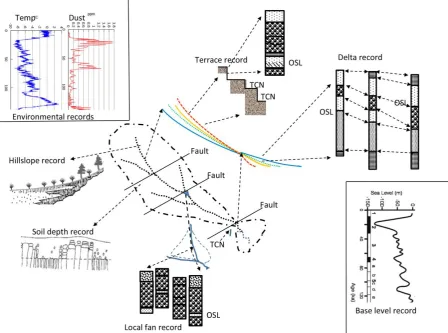
Figure 2 illustrates the type of records that could be sampled if occurring in the investigated 431
research area. These proposed multi-scale records are both erosional landscape features and 432
sedimentary records such as soil depth patterns, hillslope/colluvial records, local alluvial fan records, 433
fluvial terrace records and delta records. The latter are particularly often overlooked in field studies 434
and yet fundamental in providing an independent ‘depositional’ mirror record of the ‘erosional’ 435
record in the catchment (e.g. Whittaker et al., 2010; Forzoni et al., 2014). Comparing the catchment 436
and downstream data and partitioning the sediment budget to ensure that the budget ‘closes’ as 437
effectively as possible (although see caveats in Parsons, 2011) will improve the quality of model 438
input data. Sediment budgeting also better quantifies the field data, enabling more precise 439
evaluation of the match between modelled outputs and field observations. However, it is not always 440
easy to include downstream data. Sometimes sediment budgets cannot be closed if small-scale sinks 441
within the system store sediment over significant time periods (e.g. Blöthe and Korup, 2013), or the 442
downstream record is incomplete (e.g. Parsons, 2011) or ‘leaky’ (i.e. sediment passes through to 443
even more downstream areas such as the coast, sea or shelf). This ‘leakiness’ is hard to quantify 444
from the geological record alone (e.g. Jerolmack and Paola, 2010; Godard et al., 2014, Armitage et 445
al., 2013). Non-linearities due to hillslope – channel (dis) connectivity and events such as river 446
capture or glacial interventions would also cause a lack of a clear source to sink connectivity. In 447
relation to other record types, an example is sub-catchment outlet 10Be erosion rates which can be
448
measured to get time aggregated erosion rates (e.g. Von Blanckenburg, 2005) and combined with 449
sediment budget estimates from source sink comparisons (item 8, Table 2). 450
POS can also be applied not simply for evaluation but also for specifying initial conditions such as 451
sediment thickness and composition for each grid cell, to avoid assuming a uniform cover across the 452
catchment due to limited information. Whilst this may involve more fieldwork, it may rather involve 453
creatively using existing datasets for this new purpose. Good pedological maps can be invaluable in 454
achieving this aim (e.g. Bovy et al., 2016), as can use of geotechnical borehole data. These datasets 455
13 parallel with developments in the automatic recognition of landforms (e.g. Jones et al., 2007) from 457
DEMs, new technologies and data sources such as ground penetrating radar (GPR), other 458
geophysical surveys, LIDAR data (both airborne and scanning vertical faces) and the game changing 459
use of Structure-from Motion (SfM) to generate high resolution DSMs from aerial and UAV imagery 460
(e.g. Dabskia et al., 2017) make the collection of geomorphological and spatially distributed 461
sedimentary data much more feasible than was previously the case (Demoulin et al., 2007; Del Val et 462
al., 2015). These data can be used iteratively with remotely sensed data both before and after field 463
investigations. This spatially distributed dataset can provide information on erosional and 464
depositional landforms as well as sedimentary units (Tables 1 and 2). 465
Systematic collection of data from multiple landscape elements using a POS approach generates a 466
better description and understanding of the catchment and thus allows for a more effective 467
evaluation of model output than illustrated by Temme et al. (2017) in their Fig.4. 468
The strength of Pattern Oriented Modelling is that it recognises both the inherent (x,y,z,t) 469
uncertainties in specification of initial conditions and the non-linearity of ecological and 470
geomorphological processes and systems. Systematic Pattern Oriented Sampling will allow a more 471
systematic characterisation of the relevant landscape properties that can then be used for 472
systematic sensitivity analysis of the developed LEM. It is for example equally relevant to know 473
where sediments occur and where they do not. For landscape-evolution models, the inherent 474
(x,y,z,t) uncertainties are primarily due to DEMs, sediment thickness / characteristics and dating 475
technique uncertainties. Too often we have much data from particular locations while at the same 476
time we have almost no data outside these unique locations (often boreholes and quarries). Non-477
linearity evaluation requires approaches such as Monte Carlo sensitivity ensembles to quantify the 478
role of autogenic feedbacks in the model outcomes (Nicholas and Quine, 2010). In order to do this in 479
a meaningful way we have to quantify their spatial and temporal distributions as well as possible. 480
For example, Hajek et al. (2010) statistically define the degree of channel-belt clustering. By 481
comparing the degree of spatial clustering between channel units observed in late Cretaceous-age 482
rocks and a flume experiment, they conclude that the patterns observed could have formed as a 483
result of self-organisation within the system rather than due to external forcing (Humphrey and 484
Heller, 1995). A similar approach is taken with Quaternary age sequences by Bovy et al. (2016). 485
Similarly the strength of Pattern Oriented Sampling (POS) as illustrated in Figure 2 is that it 486
recognises the inherently stochastic nature of sediment preservation at the land surface compared 487
with at-a-point comparisons. POS therefore widens the range of possible field data that can be used 488
whilst simultaneously targeting only those data types that actually add information about the key 489
characteristics identified. It is likely that this will include areas with no sedimentary records, running 490
counter to much current geological fieldwork practice. It may also require the collection of field data 491
for evaluation of model output across the whole catchment. As such it will require an intentional 492
strategy and possibly some additional resources to observe and describe sedimentary successions 493
and landforms even in hard to access locations. We propose here various new data types and 494
patterns as useful for pattern-matching comparisons (Table 2), many of which can be quantified and 495
applied concurrently. As shown in Figure 1, identification of which of these can be used in model 496
14 POS also aids in decision making when attempting to build a robust chronology because sample 498
selection can be targeted to the key characteristics identified for the catchment as shown in Figure 499
1. For example, where depositional units are the focus, samples should be taken to enable robust 500
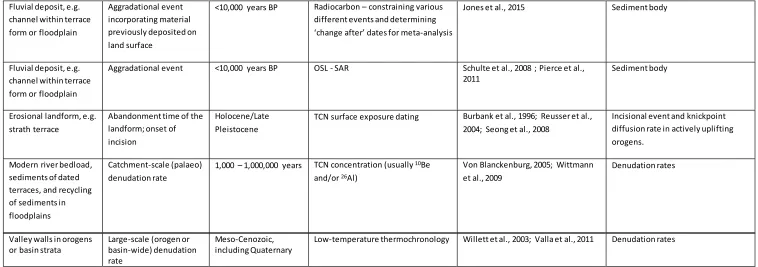
comparison between sedimentary units. This means that whilst it is necessary only to undertake 501
chronological analyses from suitable depositional settings (Table 3), chronological data should be 502
sampled both up and downstream (e.g. Chiverrell et al., 2011; Macklin et al., 2012a; Rixhon et al., 503
2011), combining vertical (successive terrace levels at a given location, e.g. Bahain et al., 2007) and 504
longitudinal (same level at multiple places along the river profile, e.g. Cordier et al., 2014) sampling. 505
This is especially important because many terraces and other fluvial sedimentary bodies are 506
diachronous features (Veldkamp and Tebbens, 2001; van Balen et al., 2010). Where stratigraphic 507
relationships are well-known, Bayesian statistics can and should be used to increase age precision. 508
We note, however, that Bayesian statistics are only helpful where units are in direct stratigraphic 509
superposition (e.g. Bayliss et al., 2015; Toms, 2013). Thus significant sediment bodies should be 510
sampled more than once, with replication at each location of ideally up to five samples. In addition, 511
as has been argued by many authors (e.g. Rixhon et al., 2017), multiple chronological methods 512
(Table 3) should be used where possible to improve robustness of the dating. Care should be taken 513
to avoid both the use of techniques beyond their reliable limits and lack of clarity about the event 514
being dated (e.g. Macklin et al., 2010). 515
In contrast, where erosional features are the key characteristic in a catchment, the determination of 516
denudation rates using Terrestrial Cosmogenic Nuclide (TCN) data can provide values with which 517
overall mean denudation rates of a catchment can be quantified (e.g. Schaller et al., 2001, 2002; Von 518
Blanckenburg, 2005; Wittmann et al., 2009). As discussed above, catchment averaged TCN data is a 519
good target for model-data comparison because such long-term, spatially-averaged data are often 520
produced by models (see for example Veldkamp et al., 2016). Low-temperature thermochronology is 521
another source of (modelled) data complementary to TCN (Table 3). It is used routinely for 522
estimating (very) long-term denudation rates in active orogens (e.g. Willett et al., 2003) or in their 523
adjacent basins. As an example, Valla et al. (2011) used thermochronology to demonstrate increased 524
incision and relief production in the Alps since the Middle Pleistocene and King et al. (2016) show 525
changes in the nature of uplift in the Himalayas. 526
Once appropriate data has been gathered, pattern-matching can and should be separated into the 527
qualitative recognition of spatial patterns and the statistically quantified distribution of specific, 528
quantifiable features (e.g. slopes, soil or sediment thickness or volume, Table 2) within model 529
output. Quantification of the goodness of fit should be applied wherever possible whilst bearing in 530
mind the appropriate spatial scale. For example, statistical analysis has been used for comparing 531
probability density functions of 14C dated Holocene flood units in New Zealand and the UK in order
532
to demonstrate interhemispheric asynchrony of centennial- and multi-centennial-length episodes of 533
river flooding related to short-term climate change (Macklin et al., 2012a). However, such meta-534
analyses sometimes aggregate data to too high a level, losing the spatial variability of the data and 535
thus data that would be crucial for evaluating POM. Quantification of goodness of fit will not always 536
be possible, but where it is, this is noted in Table 2. It should be noted that there will always be an 537
element of subjectivity/expert judgement about whether the fit is ‘good enough’. As discussed 538
above, multiple uncertainties in LEMs over geological timescales negate the uncritical use of R2
539
15
Pattern Oriented Sampling applied to specific field settings
541
Three main case study types can be distinguished where different types of field data are relevant to 542
be used in comparisons with model output. These are 1) sedimentary records where the study focus 543
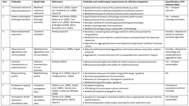
is usually on climate and anthropogenic forcing of fluvial landscape dynamics (e.g. Viveen et al., 544
2014), 2) the more erosional and morphological records that are often more focussed on tectonic 545
forcing (e.g. Demoulin et al., 2015; Beckers et al., 2015) and 3) study of long-term denudation rates 546
(e.g. Willenbring et al., 2013; Veldkamp et al., 2016). The two first categories are compared in Table 547
1 and discussed in more detail below in relation to Pattern Oriented Sampling. All case study types 548
have still unresolved challenges related to the previously discussed issues of initial topography, 549
equifinality and the separation of internal complex response from external forcing. Table 1 550
demonstrates the different data scale emphasis of the two first case study types. Table 2 gives seven 551
potential field data types that can be used to improve field-model pattern comparison. 552
A detailed discussion of the data that will be most useful in evaluating model output is important 553
because the data that is generated separately by the two endeavours (modelling and fieldwork) are 554
by nature very different. For example, field data often comprises detailed study of only a very small 555
part of the catchment (the best or ‘type’ example). Depending on the methods used to develop a 556
chronology the reconstructed depositional history of a catchment may also lack significant temporal 557
resolution, perhaps due to lack of dateable material or to large error bars. Indeed even the smallest 558
error bars possible are frequently larger than the time intervals used in model runs. In contrast, 559
model outputs have complete spatial coverage (e.g. mapped change in height / volume of sediment 560
deposited) with high temporal resolution, but often lack local detail. Variables outputted by models 561
are also different from those generated from field-based geological records – e.g. sediment and 562
discharge variations which can only be inferred from sedimentary sequences, not directly measured. 563
Whilst a combined POM-POS approach can aim to minimise these differences, it can never 564
completely eliminate them. 565
1) Sedimentary records with a focus on climate and anthropogenic forcing
566
Comparison of sedimentary field data and modelled deposition will involve integration of borehole 567
and 3-D surface data within a single system (Table 2). For example Viveen et al. (2014, Figure 3a) 568
used spatially constrained data on sediment thickness to compare with model output at multiple 569
locations within a catchment, as do Geach et al. (2015). This is not as useful as volumetric data 570
because it potentially masks the volumetric implications of variations in sediment thickness due to 571
confluences, uneven floodplain bases and scour hollows. However, borehole data is not widely 572
available from the regions in which these studies were based, so average sediment thickness had to 573
be used instead. This limits the quality of the match between field and model data in these studies 574
and means they are compared only qualitatively. It is also exemplified by the qualitative comparison 575
of modelled and observed histograms of Holocene 500-yr step sediment delivery for the Rhine and 576
the Meuse delta sediments (Erkens et al. 2006; Erkens, 2009) and catchment-data based 577
quantifications. These studies could potentially be taken further by direct comparison of the 578
modelled and observed volumes of key sediment bodies within a catchment, tightly spatially 579
constrained to ensure comparability (see item 1 in Table 2). An alternative approach to 580
16 longer time periods shows that results are highly dependent on the approach used, highlighting a 582
need to develop more standardised approaches for describing Quaternary river archives (both 583
alluvial fans and terraces - e.g. Stokes et al, 2012; Mather & Stokes, 2016; Mather et al., 2017). 584
Meta-analysis, a systematic approach to aggregating dated sedimentary units and landforms in 585
catchments (e.g. Macklin et al., 2013; Thorndycraft and Benito, 2006), can also be used in model 586
evaluation at a catchment-scale. For example, it has been used for comparing periods of aggradation 587
and quiescence found in the modelled and observed records in four adjacent upland catchments 588
(e.g. Coulthard et al., 2005; item 4, Table 2; Figure 3b). The use of consistent protocols for the 589
aggregation of data is important in order to quantify reach-scale variability in the fluvial record (cf. 590
Macklin et al., 2012b), enabling catchment-wide and regional patterns to be detected. What we 591
advocate with the Pattern Oriented Sampling however is not only aggregation but also 592
disaggregation of data to specific locations in the catchment to get a more comprehensive picture of 593
the fluvial system pattern for model comparison. More work also needs to be undertaken on how to 594
quantify the comparison of this data type because it is very dependent on the quality of the 595
chronology (item 4, Table 2). 596
2) Erosional and morphological records with a focus on tectonic forcing
597
Where the landscape is mostly erosional and the main landscape driver of interest is crustal uplift 598
(Table 1) high quality morphological data is relevant. Specific DEM-derived metrics (e.g. chi plots, 599
hypsometric integrals, geophysical relief, R/SR – e.g. Cohen et al., 2008; Perron and Roydon, 2013; 600
Demoulin et al., 2015) can be used to quantify field characteristics and integrated into a common GIS 601
software package, which will facilitate pattern-matching with model output in addition to greater 602
understanding of the systems by comparison with other basins. Data such as non-lithologically 603
controlled knickpoints or vertical spacing between fluvial terrace levels may additionally be useful 604
for model output evaluation. As Stange et al. (2014) show, the spacing, timing and tilting (i.e. 605
convergent, divergent or parallel) of exposure dated terrace forms can provide a powerful modelling 606
test of competing hypotheses about the tectonic history of a region (Item 6, Table 2; Figure 3). 607
Significantly more work is needed to quantify the match between field and modelled data in relation 608
to long profiles however. At present this is possible only subjectively. Similarly, many studies support 609
the usefulness of knickpoint mapping (item 7, Table 2). They can be used to test the validity of river-610
incision models based on the stream power law (e.g. Berlin & Anderson, 2007; Beckers et al., 2015) 611
and evaluate the role of additional controls on incision (e.g. Whittaker et al., 2007, 2008; Whittaker 612
& Boulton, 2012). TCN dating of the progression of erosion waves across drainage systems also 613
enables the two types of data to be compared (e.g. Anthony & Granger, 2007b; Rixhon et al., 2011). 614
However not all knickpoints are valid targets for model-data comparison. For example, a knickpoint 615
in a highly erodible lithology or highly resistant lithology subject to structural discontinuities (e.g. 616
Anton et al 2015) is unlikely to be useful for evaluating landscape evolution modelling of longer 617
timescales because climatic or tectonic controls on migration will be masked. In addition, other 618
tectonic factors will influence fluvial systems, for example dislocation of river courses across laterally 619
or vertically faulted landscapes, differential uplift or subsidence across substrate lithological 620
boundaries or solution driven collapse. 621
3) Promising new techniques for quantifying denudation rates
17
In situ cosmogenic-based denudation rates, which are inherently spatially and temporally averaged 623
(item 8, Table 2) provide an additional opportunity for a very powerful check on denudation rates 624
produced from landscape evolution models. They can only be used where the relevant assumptions 625
hold (i.e. relatively steady rates of sediment production over time, well-mixed sediment). To date, 626
most comparisons of numerical model output with cosmogenic denudation rates have been 627
undertaken with the aim of better understanding the robustness of the TCN signal, for example in 628
relation to different rates and styles of climate change (Schaller and Ehlers, 2006), or in basins where 629
sediment inputs to the system are dominated by landslides (Yanites et al., 2009). More recently, the 630
ability of spatial analysis of such denudation rates to improve understanding of transient response to 631
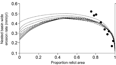
a tectonic perturbation has been effectively shown by Willenbring et al. (2013), with an acceptable 632
match between independently modelled and cosmogenic-based basin-wide denudation rates (Figure 633
4). More recently Veldkamp et al., (2016) used fluvial terrace properties (thickness and timing of 634
deposition/erosion for specific locations) to calibrate a longitudinal profile model. After an elaborate 635
stepwise calibration and sensitivity analysis the derived temporal landscape erosion (sedimentary 636
delivery) rates were compared with measured 10Be catchment denudation rates (Schaller et al.,
637
2002), proving to be comparable both in rate magnitudes and timing. We therefore propose that this 638
approach has reached sufficient maturity that it should be used more widely in future studies, by 639
using cosmogenic-based denudation rates as a means to evaluate landscape evolution modelling 640
over timescales of 102-105 years.
641
With regard to intra-catchment pattern identification, TCN-based denudation rates can address this 642
by sampling streams of different orders. Differences between catchments can highlight a specific 643
intrinsic control such as lithology, steepness, a climatic gradient or different tectonic histories (Von 644
Blanckenburg, 2005), which are also key questions often addressed in landscape evolution modelling 645
studies. TCN-based denudation rates help to constrain such controls across a wide range of spatial 646
scales. However, one must bear in mind that a steady state assumption is intrinsic when deriving 647
TCN-denudation rates, such that applications of this method to non-steady state settings should be 648
exercised with care. Non-steady state settings are most common in catchments prone to mass-649
wasting processes, such as landsliding, where most of the sediments leaving the catchment may 650
originate from a small area and there is therefore incomplete sediment mixing between hillslope and 651
channels, as recorded in differing cosmogenic nuclide concentrations (Small et al., 1997; Norton et 652
al., 2010; Binnie et al., 2006; Savi et al., 2013). Large contrasts in lithology within a catchment may 653
also cause these assumptions to be violated (von Blanckenburg, 2005). In practice, although such 654
situations should be avoided when they are obviously present, they are rare and in many cases TCN 655
have proven to record robust denudation rates over wide ranges of climatic and tectonic settings 656
(Table 2). 657
Recommendations
658
Landscape evolution models have moved away from purely theoretical research questions 659
addressed in synthetic landscapes towards answering specific research questions in particular 660
catchments. This brings into sharp relief the nature of the field data that enables effective evaluation 661
of model outputs. We have argued above that the current practise of field data collection does not 662
18 Firstly, researchers need to be aware that landscape evolution models are qualitatively different 664
from other earth surface process models commonly used in the environmental sciences. They 665
operate over longer geological time periods, with sparser datasets and a different purpose. Research 666
questions usually seek explanation rather than numerical prediction, using an insightful 667
simplification approach where minimum numbers of parameters are used. Instead of seeking an 668
optimum set of parameters, different model runs often explore their relative importance and the 669
effects of changing their amplitude. Whilst such forward modelling can result in equifinality, we 670
argue that this should be embraced as narrowing down the plausible set of events that have 671
occurred in the catchment, even if not converging on a single outcome. Indeed such convergence 672
might suggest a greater level of certainty than is actually present and thus be misleading. 673
Secondly, we advocate the use of a quantitative pattern-matching approach for field-model 674
evaluation such as that often used in ecological studies. Recognizing that fluvial landscape evolution 675
modelling is also a pattern-oriented modelling (POM) approach (Grimm and Railsback, 2012), 676
generating geological field data that is comparable with model output will require adaptation of 677
fieldwork strategies using pattern-oriented sampling (POS). This sampling should focus only on data 678
that provides information about identified key characteristics of the catchment (Figure 1). This will 679
embrace a wider range of data types overall (Figure 2), but not increase the burden of data 680
collection for study of a specific catchment. A number of suitable data targets for such an approach 681
are outlined in Table 2 and exemplified in Figures 3-5 and related text. 682
We have shown that Pattern Oriented Sampling is starting to be applied in some cases. However, we 683
believe that the community should more generally apply these principles in a structured way. Our 684
aim as FACSIMILE is to facilitate a research approach that compares this wider range of field data 685
with model output from a range of model types. Given that it is neither possible nor desirable to 686
model all systems, we are in the process of working on a specific field catchment where initial 687
pattern-matching model-data comparisons can be undertaken to determine further which 688
approaches are most useful. 689
Acknowledgements
690
The authors are grateful to the Faculty of Geo-Information Science and Earth Observation of the 691
University of Twente who provided support for two workshops during which these ideas were 692
developed. We also thank three anonymous referees and the Associate Editor Professor Stuart Lane 693
whose comments greatly clarified our thinking on these matters. 694
References
695
Adamson KR, Woodward JC, Hughes, PD. 2014. Glaciers and rivers: Pleistocene uncoupling in a 696
Mediterranean mountain karst. Quaternary Science Reviews 94: 28-43. 697
Anderson RS, Repka JL, Dick GS. 1996. Explicit treatment of inheritance in dating depositional surface 698
using in situ 10Be and 26Al. Geology24: 47-51.