On Eulerian equilibria in K order approximation of the gyrostat in the three body problem

OF THE GYROSTAT IN THE THREE-BODY PROBLEM

Received 9 June 2006; Revised 21 September 2006; Accepted 9 November 2006

We consider the noncanonical Hamiltonian dynamics of a gyrostat in the three-body problem. By means of geometric-mechanics methods we study the approximate Poisson dynamics that arises when we develop the potential in series of Legendre and truncate this in an arbitrary orderk. Working in the reduced problem, the existence and number of equilibria, that we denominate of Euler type in analogy with classic results on the topic, are considered. Necessary and sufficient conditions for their existence in an approximate dynamics of orderkare obtained and we give explicit expressions of these equilibria, use-ful for the later study of the stability of the same ones. A complete study of the number of Eulerian equilibria is made in approximate dynamics of orders zero and one. We ob-tain the main result of this work, the number of Eulerian equilibria in an approximate dynamics of orderkfork≥1 is independent of the order of truncation of the potential if the gyrostatS0is close to the sphere. The instability of Eulerian equilibria is proven for any approximate dynamics if the gyrostat is close to the sphere. In this way, we generalize the classical results on equilibria of the three-body problem and many of those obtained by other authors using more classic techniques for the case of rigid bodies.

Copyright © 2006 J. A. Vera and A. Vigueras. This is an open access article distributed under the Creative Commons Attribution License, which permits unrestricted use, dis-tribution, and reproduction in any medium, provided the original work is properly cited. 1. Introduction

In the study of configurations of relative equilibria by differential geometry methods or by more classical ones, we will mention here the papers of Wang et al. [8], about the problem of a rigid body in a central Newtonian field; Maciejewski [3], about the problem of two rigid bodies in mutual Newtonian attraction. These papers have been generalized to the case of a gyrostat by Mondejar and Vigueras [4] to the case of two gyrostats in mutual Newtonian attraction.

Hindawi Publishing Corporation

International Journal of Mathematics and Mathematical Sciences Volume 2006, Article ID 72978, Pages1–17

For the problem of three rigid bodies we would like to mention that Vidyakin [7] and Dubochine [1] proved the existence of Euler and Lagrange configurations of equilibria when the bodies possess symmetries; Zhuravlev and Petrutskii [9] made a review of the results up to 1990.

In Vera [5] and a recent paper of Vera and Vigueras [6] we study the noncanonical Hamiltonian dynamics ofn+ 1 bodies in Newtonian attraction, wheren of them are rigid bodies with spherical distribution of mass or material points and the other one is a triaxial gyrostat.

Let us remember that a gyrostat is a mechanical systemS, composed of a rigid body

S, and other bodiesS(deformable or rigid) connected to it, in such a way that their relative motion with respect to its rigid part do not change the distribution of mass of the total systemS, (see Leimanis [2] for details).

In this paper, we taken=2 and as a first approach to the qualitative study of this sys-tem, we describe the approximate dynamics that arises in a natural way when we take the Legendre development of the potential function and truncate this until an arbitrary or-der. We give global conditions on the existence of relative equilibria and in analogy with classic results on the topic, we study the existence of relative equilibria that we will de-nominate of Euler type in the case in whichS1,S2are spherical or punctual bodies andS0 is a gyrostat. Necessary and sufficient conditions for their existence in a approximate dy-namics of orderkare obtained and we give explicit expressions of these equilibria, useful for the later study of the stability of the same ones. A complete study of the number of Eulerian equilibria is made in approximate dynamics of orders zero and one. The num-ber of Eulerian equilibria in an approximate dynamics of orderkfork >1 is independent of the order of truncation of the potential if the gyrostatS0is close to the sphere. The instability of Eulerian equilibria is proven for any approximate dynamics if the gyrostat is close to the sphere. The analysis is done in vectorial form avoiding the use of canonical variables and the tedious expressions associated with them.

We should notice that the studied system has potential interest both in astrodynamics (dealing with spacecraft) as well as in the understanding of the evolution of planetary systems recently found (and more to appear), where some of the planets may be modeled like a gyrostat rather than a rigid body. In fact, the equilibria reported might be well compared with the ones taken for the “parking areas” of the space missions (GENESIS, SOHO, DARWIN, etc.) around the Eulerian points of the Sun-Earth and the Earth-Moon systems.

To finish this introduction, we describe the structure of the article. The paper is orga-nized in five sections, two appendices, and the bibliography. In these sections we study the equations of motion, Casimir function and integrals of the system, the relative equi-libria and the existence of Eulerian equiequi-libria in an approximate dynamics of orderk, in particular the study of the bifurcations of Eulerian equilibria in an approximate dynamics of orders zero and one.

2. Equations of motion

λ

μ

Ωe

Figure 2.1. Gyrostat in the three-body problem.

For u, v∈R3_{, u·v is the dot product,|u|is the Euclidean norm of the vector u, and} u×v is the cross-product. IR3is the identity matrix and 0 is the zero matrix of order three.

Let z=(Π,λ, pλ,μ, pμ)∈R15be a generic element of the twice reduced problem obtained using the symmetries of the system, where Π=IΩ+ lr is the total rotational angular momentum vector of the gyrostat,I=diag(A,B,C) is the diagonal tensor of inertia of the gyrostat, andΩis the angular velocity ofS0in the body frame,J, which is attached to its rigid part and whose axes have the direction of the principal axes of inertia ofS0. The vector lris the gyrostatic momentum that we suppose constant and is given by lr= (0, 0,l). The elementsλ,μ, pλ, and pμ are, respectively, the barycentric coordinates and the linear momenta expressed in the body frameJ(seeFigure 2.1).

The twice reduced Hamiltonian of the system, obtained by the action of the group SE(3), has the following expression:

Ᏼ(z)=pλ 2

2g1 + _pμ2

2g2 + 1 2ΠI

−1_Π−lr·I−1_{Π+ᐂ (2.1)}

with

M2=m1+m2, M1=m1+m2+m0,

g1=m1m2

M2 ,

g2=m0M2

M1 ,

(2.2)

withᐂbeing the potential function of the system given by the formula

ᐂ(λ,μ)= −

Gm1m2 |λ| +

S0

Gm1dm(Q) _{Q +μ+}

m2

M2

λ+

S0

Gm2dm(Q) _{Q +μ−}

m1

M2

λ

. (2.3)

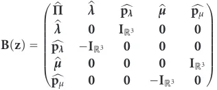
Let M=R15_{, and we consider the manifold (M,{·,·},Ᏼ), with Poisson brackets{·,·}} defined by means of the Poisson tensor

B(z)= ⎛ ⎜ ⎜ ⎜ ⎜ ⎜ ⎜ ⎝

Π _λ pλ μ pμ

λ 0 IR3 0 0

pλ −IR3 0 0 0

μ 0 0 0 IR3

pμ 0 0 −IR3 0

⎞ ⎟ ⎟ ⎟ ⎟ ⎟ ⎟ ⎠

In B(z),v is considered to be the image of the vector v ∈R3_{by the standard} isomor-phism between the Lie AlgebrasR3_{andso(3), that is,}

v=

⎛ ⎜ ⎝

0 −v3 v2

v3 0 −v1

−v2 v1 0 ⎞ ⎟

⎠. (2.5)

The equations of the motion are given by the following expression:

dz

dt =

z,Ᏼ(z) (z)=B(z)∇zᏴ(z), (2.6)

where∇zf is the gradient of f ∈C∞(M) with respect to an arbitrary vector z.

Developing{z,Ᏼ(z)}, we obtain the following group of vectorial equations of the mo-tion:

dΠ

dt =Π×Ω+λ×∇λᐂ+μ×∇μᐂ, dλ

dt =

pλ

g1+λ×Ω,

dpλ

dt =pλ×Ω−∇λᐂ,

dμ dt =

pμ

g2 +μ×Ω,

dpμ

dt =pμ×Ω−∇μᐂ.

(2.7)

Important elements of B(z) are the associate Casimir functions. We consider the total angular momentum L given by

L=Π+λ×pλ+μ×pμ. (2.8)

Then the following result is verified (see Vera and Vigueras [6] for details).

Proposition 2.1. Ifϕis a real smooth function not constant, thenϕ(|L|2_{/2) is a Casimir} function of the Poisson tensor B(z). Moreover Ker B(z)= ∇zϕ. Also,dL/dt=0, that is to say the total angular momentum vector remains constant.

2.1. Approximate Poisson dynamics. To simplify the problem we assume that the gyro-statS0is symmetrical around the third axis of inertiaOZand with respect to the plane

OXY beingOX,OY,OZ are the coordinated axes of the body frame J. If the mutual distances are bigger than the individual dimensions of the bodies, then we can develop the potential in fast convergent series. Under these hypotheses, we will be able to carry out a study of equilibria in different approximate dynamics.

Applying the Legendre development of the potential, we have

ᐂ(λ,μ)= −

Gm1m2 |λ| +

∞

i=0

Gm1A2i _μ+

m2

M2

λ2i+1+ ∞

i=0

Gm2A2i _μ−

m1

M2

λ2i+1

, (2.9)

Definition 2.2. We call approximate potential of orderkto the following expression:

ᐂk(λ,μ)= −

Gm1m2 |λ| +

k

i=0

Gm1A2i _μ+

m2

M2

λ2i+1+ k

i=0

Gm2A2i _μ−

m1

M2

λ2i+1

. (2.10)

It is easy to demonstrate the following lemmas.

Lemma 2.3. Given the approximate potential of orderk,

∇λᐂk=Gm_|λ1_|m32λ+

Gm1m2

M2 k

i=0

μ+m2

M2

λ(2i+ 1)A2i _μ+

m2

M2

λ2i+3

−Gm1m2

M2 k

i=0

μ−m1

M2

λ(2i+ 1)A2i _μ−

m1M2λ2i+3 ,

∇μᐂk=Gm1 k

i=0

μ+m2M2λ(2i+ 1)A2i _μ+

m2

M2

λ2i+3 +Gm2 k

i=0

μ−m1M2λ(2i+ 1)A2i _μ−

m1

M2

λ2i+3 . (2.11)

The following identities are verified

∇λᐂk=A11λ+A12μ, ∇μᐂk=A21λ+A22μ (2.12)

being

A11(λ,μ)=Gm1m2 |λ|3 +

Gm1m22

M22 _k

i=0

βi _μ+ m2 M2

λ2i+3

+Gm 2 1m2

M2 2

_k

i=0

βi _μ− m1 M2

λ2i+3

,

A12(λ,μ)=Gm1m2

M2 _k

i=0

βi _μ+ m2 M2

λ2i+3− k

i=0

βi _μ− m1 M2

λ2i+3

,

A22(λ,μ)=Gm1 _k

i=0

βi _μ+ m2 M2

λ2i+3

+Gm2 _k

i=0

βi _μ− m1 M2

λ2i+3

,

A21(λ,μ)=A12(λ,μ)

(2.13)

Definition 2.4. Let M=R15_{and the manifold (M,{·,·},Ᏼk), with Poisson brackets{·,·},} defined by means of the Poisson tensor (2.4). We call approximate dynamics of orderkto the differential equations of motion given by the following expression:

dz

dt =

z,Ᏼk(z), (z)=B(z)∇zᏴk(z) (2.14)

being

Ᏼk(z)=|pλ|2 2g1 +

|pμ|2 2g2 +

1 2ΠI

−1_Π−lr·I−1_{Π+ᐂk(λ,μ). (2.15)}

2.1.1. Integrals of the system. On the other hand, it is easy to verify that

∇z

|Π|2_{B(z)∇zᏴ0(z)=0 (2.16)}

and similarly when the gyrostat is of revolution ∇z

Π3

B(z)∇zᏴk(z)=0, (2.17)

whereπ3is the third component of the rotational angular momentum of the gyrostat. It is verified the following result.

Theorem 2.5. In the approximate dynamics of order 0,|Π|2_{is an integral of motion and} also when the gyrostat is of revolutionπ3is another integral of motion.

2.2. Relative equilibria. The relative equilibria are the equilibria of the twice reduced problem whose Hamiltonian function is obtained in Vera and Vigueras [6] for the case

n=2. If we denote by ze=(Πe,λe, pe_λ,μe_{, p}e

μ) a generic relative equilibrium of an approx-imate dynamics of orderk, then this verifies the equations

Πe×Ωe+λe×

∇λᐂke+μe×

∇μᐂke=0,

pe_λ

g1 +λ e_×Ω

e=0, pe_λ×Ωe=∇λᐂke, pe

μ

g2 +μ e_×Ω

e=0, peμ×Ωe=

∇μᐂke.

(2.18)

Also by virtue of the relationships obtained in Vera and Vigueras [6], we have the following result.

Lemma 2.6. If ze=(Πe,λe, pe_λ,μe, peμ) is a relative equilibrium of an approximate dynamics of orderk, the following relationships are verified:

_Ωe2 λe2

−λe_·Ω e

2 = 1

g1

λe_·∇ λᐂke

, _Ωe2

μe2

−μe_·Ω e

2 = 1

g2

μe_·∇ μᐂke

.

The last two previous identities will be used to obtain necessary conditions for the existence of relative equilibria in this approximate dynamics.

We will study certain relative equilibria in the approximate dynamics supposing that the vectorsΩe,λe,μesatisfy special geometric properties.

Definition 2.7. zeis an Eulerian relative equilibrium in an approximate dynamics of order

kwhenλeandμe_{are proportional andΩ}

eis perpendicular to the straight line that they generate.

Remark 2.8. The previous hypotheses simplify the conditions ofLemma 2.6. In a next paper we will study the possible “inclined” relative equilibria, in whichΩeform an angle

α =0 andπ/2 with the vectorλe.

From the equations of motion, the following property is deduced.

Proposition 2.9. In a Eulerian relative equilibrium for any approximate dynamics of

ar-bitrary order, moments are not exercised on the gyrostat.

Next we obtain necessary and sufficient conditions for the existence of Eulerian relative equilibria.

3. Relative equilibria of Euler type

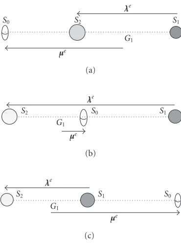
According to the relative position of the gyrostatS0with respect toS1andS2, there are three possible equilibrium configurations (seeFigure 3.1): (a)S0S2S1, (b)S2S0S1, and (c)

S2S1S0.

3.1. Necessary condition of existence

Lemma 3.1. If ze=(Πe,λe, peλ,μe, peμ) is a relative equilibrium of Euler type, then for the configurationS0S2S1,

μe₊ m1

M2λ

e_=λe_+μe₋m2

M2λ

e_{. (3.1)}

In a similar way, for the configurationS2S0S1,

_λe_=μe₋m1

M2λ

e_+μe₊ m2

M2λ

e_{. (3.2)}

Finally, for the configurationS2S1S0, μe₋m2

M2λ

e_=μe₊m1

M2λ

e_+λe_{. (3.3)}

S0 S2 S1

λe

G1

μe

(a)

S2 S0 S1

λe

G1

μe

(b)

S2 S1 S0

λe

G1

μe

(c)

Figure 3.1. Eulerian configurations.

approximate dynamics of orderk, we have

g1Ωe2λe2=λe·

∇λᐂke, g2Ωe2μe2=μe·

∇μᐂke,

μe₋m1

M2λ

e_=ρλe_{, μ}e₊ m2

M2λ

e_{=(1 +ρ)λ}e_{, μ}e₌

(1 +ρ)m1+ρm2

M2 λ

e_, (3.4)

whereρ∈(0, +∞) in the case (a),ρ∈(−1, 0) in the case (b), andρ∈(−∞,−1) in the case (c). And it is possible to obtain the following expressions:

∇λᐂke= f1(ρ)λe,

∇μᐂk)e=f2(ρ)λe, (3.5)

where

f1(ρ)=Gm1m2 _λe3 +

Gm1m2

M2 k

i=0

βi _λe2i+3

_{1 +ρ} |1 +ρ|2i+3−

ρ

|ρ|2i+3

,

f2(ρ)= k

i=0

Gβi _λe2i+3

_{m1(1 +ρ)} |1 +ρ|2i+3+

m2ρ |ρ|2i+3

.

Restricting us to the case (a) we have

f1(ρ)=Gm 1m2 λe3 +

Gm1m2

M2 _k

i=0

βi _λe2i+3

₁

(1 +ρ)2i+2− 1

ρ2i+2

,

f2(ρ)= k

i=0

Gβi _λe2i+3

_m

1 (1 +ρ)2i+2+

m2

ρ2i+2

.

(3.7)

Now, from the identities

λe_{·∇λᐂk)e=λ}e2

f1(ρ), μe_·∇μᐂk e=

(1 +ρ)m1+ρm2

M2

_λe2

f2(ρ) (3.8)

we deduce the following equations: _Ωe2

= f1(_gρ) 1 ,

_Ωe2

=_g M2f2(ρ) 2

(1 +ρ)m1+ρm2

. (3.9)

Then for a relative equilibrium of Euler typeρmust be a positive real root of the following equation:

m0m1+m2(1 +ρ)m1+ρm2f1(ρ)=m1m2m0+m1+m2f2(ρ). (3.10)

We summarize all these results in the following proposition.

Proposition 3.2. If ze=(Πe,λe, pe_λ,μe, peμ) is an Eulerian relative equilibrium in the con-figuration S0S2S1, (3.10) has, at least, a positive real root; where the functions f1(ρ) and

f2(ρ) are given by (3.7) and the modulus of the angular velocity of the gyrostat is _Ωe2

= f1(_gρ)

1 . (3.11)

Remark 3.3. If a solution of relative equilibrium of Euler type exists, in an approximate dynamics of orderk, fixing|λe|, (3.10) has positive real solutions. The number of real roots of (3.10) will depend, obviously, on the numerous parameters that exist in our system. Similar results would be obtained for the other two cases.

3.2. Sufficient condition of existence. The following proposition indicates how to find solutions of (2.18).

Proposition 3.4. Fixing|λe_{|, letρ be a solution of (3.10) where the functions f1(ρ) and}

f2(ρ) are given for the case (a) as (3.7) then ze=(Πe,λe, pe_λ,μe, peμ), given by λe_=λe_{, 0, 0, μ}e_=μe_{, 0, 0, Ω}

e=

0, 0,ωe

, pe

λ=0,g1ωeλe, 0

, pe

μ=0,g2ωeμe, 0

, Πe=

0, 0,Cωe+l

where

μe₌

(1 +ρ)m1+ρm2

M2 λ

e_{, ω}2 e=

f1(ρ)

g1

, (3.13)

is a solution of relative equilibrium of Euler type, in an approximate dynamics of orderkin the configurationS0S2S1. The total angular momentum of the system is given by

L=0, 0,Cωe+l+g1ωeλe+g2ωeμe, (3.14) wherelis the gyrostatic momentum.

Let us see the existence and number of solutions for the approximate dynamics of or-ders zero and one, respectively. For superior order it is possible to use a similar technical.

4. Eulerian equilibria in an approximate dynamics of orders zero and one

For the configurationS0S2S1, in an approximate dynamics of order zero, we have

f1(ρ)=Gm 1m2 λe3

1 +m0

M2

₁

(1 +ρ)2− 1

ρ2

,

f2(ρ)= Gm0 _λe3

_m

1 (1 +ρ)2+

m2

ρ2

.

(4.1)

Equation (3.10) is equivalent to the following polynomial equation:

m1+m2

ρ5_+3m 1+ 2m2

ρ4_+3m 1+m2

ρ3

−3m0+m2

ρ2−3m0+ 2m2

ρ−m0+m2

=0. (4.2)

This equation has an unique positive real solution, then in this case for the approxi-mate dynamics of order zero, there exists a unique relative equilibrium of Euler type.

On the other hand, one has _Ωe2

=G

m1+m2 _λe3

1 + m0

m1+m2

1 (1 +ρ)2−

1

ρ2

, (4.3)

ρbeing the only one positive solution of (4.2).

The following proposition gathers the results about relative equilibria of Euler type in an approximate dynamics of order zero in any of the previously mentioned cases (a), (b), or (c).

Proposition 4.1. (1) Ifρis the unique positive root of (4.2) with|Ωe|2being expressed as (4.3), then ze=(Πe,λe, pe_λ,μe, peμ), given by

λe_=λe_{, 0, 0, μ}e_=μe_{, 0, 0, Ω}

e=0, 0,ωe, pe_λ=0,g1ωeλe, 0, peμ=0,g2ωeμe, 0, Πe=0, 0,Cωe+l,

(4.4)

(2) Ifρ∈(−1, 0) is the unique root of the equation

m1+m2ρ5+3m1+ 2m2ρ4+3m1+m2ρ3 +3m0+ 2m1+m2

ρ2_+3m 0+ 2m2

ρ+m0+m2

=0 (4.5)

with

_Ωe2 =G

m1+m2 _λe3

1 + m0

m1+m2 ₁

ρ2− 1 (1 +ρ)2

, (4.6)

then ze=(Πe,λe, pe_λ,μe, peμ), given by

λe_=λe_{, 0, 0, μ}e_=μe_{, 0, 0, Ω} e=

0, 0,ωe

, pe_λ=0,g1ωeλe, 0

, pe_μ=0,g2ωeμe, 0

, Πe=

0, 0,Cωe+l

, (4.7)

is the unique solution of relative equilibrium of Euler type in the configurationS2S0S1. (3) Ifρ∈(−∞,−1) is the unique root of the equation

m1+m2ρ5+3m1+ 2m2ρ4+2m0+ 3m1+m2ρ3 +3m0+m2

ρ2_+3m 0+ 2m2

ρ+m0+m2

=0 (4.8)

with

_Ωe2 =G

m1+m2 _λe3

1 + m0

m1+m2 ₁

ρ2+ 1 (1 +ρ)2

, (4.9)

then ze=(Πe,λe, pe_λ,μe, peμ), given by

λe_=λe_{, 0, 0, μ}e_=μe_{, 0, 0, Ω} e=

0, 0,ωe

, pe_λ=0,g1ωeλe, 0

, pe_μ=0,g2ωeμe, 0

, Πe=

0, 0,Cωe+l

, (4.10)

is the unique solution of relative equilibrium of Euler type in the configurationS2S1S0. Remark 4.2. Ifm0→0, then|Ωe|2=G(m1+m2)/|λe|3and the equations that determine the Eulerian equilibria are the same ones of the restricted three-body problem.

1.2

1

0.8

0.6

0.4

0.2

0

β1

0 0.05 0.1 0.15 0.2 0.25 0.3 ξ1 ρ0

ρ

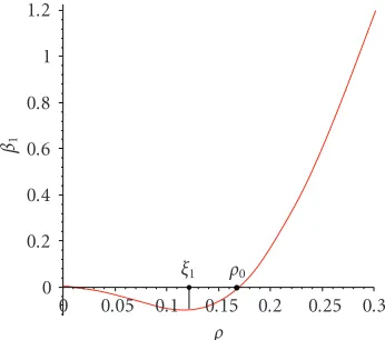
Figure 4.1. FunctionR1(ρ).

real roots of the polynomial

p1(ρ)=m0a2

m1+m2

ρ9_+m 0a2

5m1+ 4m2

ρ8_+m 0a2

10m1+ 6m2

ρ7

+ 3m0a2

3m1+m2−m0

ρ6+ 3m0a2

m1−m2−3m0

ρ5

−6m0m2a2+ 10m20a2+β1

m1+m2+ 5m0

ρ4

−4m0m2a2+ 5m20a2+β1

10m0+ 4m2

ρ3

−m0m2a2+m20a2+β1

6m2+ 10m0

ρ2

−β1

5m0+ 4m2

ρ−β1

m0+m2

,

(4.11)

wherea= |λe|andβ1=3(C−A)/2,CandAbeing the principal moments of inertia of the gyrostat.

To study the positive real roots of this equation, after a detailed analysis of the same one, it can be expressed in the following way:

β1=R1(ρ)=

m0a2ρ2(ρ+ 1)2p0(ρ)

q0(ρ) , (4.12)

Where β1=3(C−A)/2, p0 is the polynomial of grade five that determines the relative equilibria in the approximate dynamics of order 0, that is given by formula (4.2), and the polynomialq0comes determined by the following expression:

q0(ρ)=m1+m2+ 5m0

ρ4_+4m

2+ 10m0

ρ3

+6m2+ 10m0

ρ2+4m2+ 5m0

ρ+m0+m2

. (4.13)

The rational functionR1(ρ), for any value ofm0,m1,m2, always presents a minimum

ξ1 located among 0 andρ0, with this last value being the only one positive zero of the polynomialp0(ρ).

Proposition 4.3. In the approximate dynamics of order one, if the gyrostatS0is prolate (β1<0), the following hold:

(1)β1< R1(ξ1), then relative equilibria of Euler type do not exist.

(2)β1=R1(ξ1), then there exists an only relative equilibrium of Euler type.

(3)R1(ξ1)< β1<0, then two 1-parametric families of relative equilibria of Euler type exist.

IfS0is oblate (β1>0), then there exists a unique 1-parametric family of relative equilibria of Euler type.

Similarly for the configurationS2S0S1we obtain the following result (see FiguresA.1 andA.2).

Proposition 4.4. In the approximate dynamics of order one, ifm1 =m2and the gyrostat

S0 is oblate, then there exists an unique 1-parametric family of relative equilibria of Euler type; on the other hand, if the gyrostatS0is prolate and we have:

(1)β1< R1(ξ1), then there exists an unique 1-parametric family of relative equilibria of Euler type.

(2)β1=R1(ξ1), then two relative equilibria of Euler type exist.

(3)R1(ξ1)< β1<0, then three 1-parametric families of relative equilibria of Euler type exist. Ifm1=m2andS0is oblate, then relative equilibria of Euler type do not exist; but ifS0is prolate we have:

(4)R1(−1/2)< β1<0, then two 1-parametric families of relative equilibria of Euler type exist.

(5)β1=R1(−1/2), there exists an only equilibrium of Euler type. (6)β1< R1(−1/2), then relative equilibria of Euler type do not exist.

The results for the configurationS2S1S0are similar to that of the configurationS0S2S1. 4.1.1. Number of Eulerian equilibria in an approximate dynamics of orderk. In the approx-imate dynamics of orderk, the polynomialpk(ρ), that determines the Eulerian equilibria has degree 5 + 4k. Similar results to the previous ones show

pk(ρ)=m0a2ρ2(ρ+ 1)2pk−1(ρ) +βkqk−1(ρ) (4.14)

withqk−1(ρ) being a positive polynomial. In general, for usual celestial bodies,βk≈0 fork >1. Using a recurrent reasoning and applying the implicit function theorem, the number of Eulerian equilibria in the approximate dynamics of order k is the same as that of the approximate dynamics of order one. Ifβkis not close to zero, for certaink, a particular analysis of the equationpk(ρ) should be made.

4.2. Stability of Eulerian relative equilibria. The tangent flow of (2.7) in the equilibrium zecomes given by

dδz

dt =U

zeδz (4.15)

The characteristic polynomialU(ze) has the following expression:

p=λλ2_+Φ2_λ4_+mλ2_+nλ8_+pλ6_+qλ4_+rλ2_{+s (4.16)}

withΦ=((C−A)ωe+l)/A, where the coefficients that intervene in the previous polyno-mial are functions of the parameters of the problem andρbeingρthe root of (3.10). 4.2.1. Order-zero approximate dynamics. The characteristic polynomial (4.16) ofU(ze) simplifies to

p=λ3_λ2_+Φ2_λ2_+ω2 e

2

λ2_+pλ4_+qλ2_{+r (4.17)}

with coefficients expressed inAppendix B.

Ifp≥0,q≥0,r≥0,q2_{−4r≥0, then zeis spectrally stable. These conditions are not} verified sincer <0.

Proposition 4.5. If ze is the only relative equilibrium in the configurationS0S2S1 of the zero-order approximate dynamics, then this is unstable.

4.2.2. Order-one approximate dynamics. We will analyze the case in which the gyrostat is close to sphere. In this caseC−A≈0, then applying the implicit function theorem, zeis unstable.

IfC−Ais not close to zero, the coefficients of the polynomial (4.16) have very com-plicated expressions. Numeric calculations prove that there exist, for certain values of the parameterC−A, linear stable Eulerian relative equilibria (see Vera [5] for details).

These results are equally valid for the configurationsS2S0S1andS2S1S0.

5. Conclusions and future works

The approximate Poisson dynamics of a gyrostat (or rigid body) in Newtonian interac-tion with two spherical or punctual rigid bodies is considered. We give global condiinterac-tions on the existence of Eulerian equilibria and in analogy with classic results on the topic, we study the existence of equilibria that we denominate of Euler type in the case in which

S1,S2are spherical or punctual bodies andS0is a gyrostat. Necessary and sufficient con-ditions for their existence in a approximate dynamics of orderk are obtained and we give explicit expressions of these equilibria, useful for the later study of the stability of the same ones. A complete study of the number of Eulerian equilibria is made in approximate dynamics of orders zero and one. The number of Eulerian equilibria in an approximate dynamics of orderkfork >1 is independent of the order of truncation of the potential if the gyrostatS0is close to the sphere. The instability of Eulerian equilibria is proven for any approximate dynamics if the gyrostat is close to the sphere

β1

ρ0

1

ρ1

ρ 0

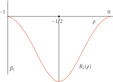
Figure A.1. FunctionR1(ρ) form1 =m2.

β1 1

1/2

R2(ρ) ρ

0

Figure A.2. FunctionR1(ρ) form1=m2.

Appendices

A. The functionR1(ρ) in approximate dynamics of order one for the configurationS2S0S1

B. Coefficients of the characteristic polynomial in Eulerian relative equilibria

The coefficients of the characteristic polynomial (4.17) are

ω2 e =

Gm2+m1

ρ4_+2m 1+ 2m2

ρ3_+m 2+m1

ρ2_−2m 0ρ−m0

λ3

e(1 +ρ)2ρ2

,

p=G

m2+ 4m0+m1

ρ3_+3m 2+ 6m0

ρ2_+4m 0+ 3m2

ρ+m0+m2

(1 +ρ)3_ρ3_λ3 e

,

q=G−2m1ρ4m2+

−2m0m1+m21+m22−2m1m2−2m0m2

ρ3

+3m22+m1m2−6m0m1

ρ2+−m1m2+ 3m22+ 2m0m2−4m0m1

ρ

+m22−m0m1+m0m2−m1m2

(1 +ρ)3ρ3λ3e

,

r=G2

a1ρ4+a2ρ4+a3ρ2+a4ρ+a5

(1 +ρ)8_ρ8_λ9 e

.

B.1. Coefficientsai(i=1,. . ., 5)

a1= −42m72m1−48m72m0−147m26m21−336m62m1m0−129m62m20 −207m52m31−782m52m21m0−673m25m1m20−81m52m30−150m42m41 −869m4

2m31m0−1325m42m21m20−378m42m1m04−64m32m51 −513m3

2m41m0−1270m32m31m20−702m32m21m03−14m22m61 −165m22m51m0−610m22m41m02−648m22m31m30−24m2m61m0 −119m2m51m02−297m2m41m30+ 2m61m20−54m51m30.

a2= −60m72m1−54m72m0−243m26m21−474m62m1m0−173m62m20 −399m5

2m31−1345m52m21m0−999m52m1m20−135m52m30−329m42m41 −1846m42m31m0−2223m42m21m20−648m42m1m30 −138m32m51 −1364m3

2m41m0−2506m32m31m20−1242m32m21m03−24m22m61 −536m2

2m51m0−1530m22m41m20−1188m22m31m30−90m2m61m0 −477m2m51m02−567m2m41m30−56m61m20−108m51m30.

a3= −42m72m1−36m72m0−183m26m21−342m62m1m0−93m62m20 −349m52m31−1097m52m21m0−630m25m1m20−81m52m30−358m42m41 −1776m4

2m31m0−166m42m21m20−405m42m1m03−189m32m51 −1614m32m41m0−2256m32m31m02−810m32m21m30−31m22m61 −827m2

2m51m0−1683m22m41m20−810m22m31m30−6m2m71 −228m2m61m0−666m2m51m02−405m2m41m30−30m71m0 −81m51m30−111m61m20.

a4= −12m72m1−12m72m0−56m26m21−114m62m1m0−24m62m20 −130m52m31−387m52m21m0−162m52m1m02−179m42m41 −687m4

2m31m0−432m42m21m20−140m32m51−693m32m41m0 −588m3

2m31m20−52m22m61−387m22m51m0−432m22m14m20−6m2m71 −108m2m61m0−162m2m51m20−12m71m0−24m61m20.

a5= −m0+m218m0m62+ 12m1m62+ 94m52m0m1+ 36m21m52

+ 81m42m20m1+ 168m42m0m12+ 42m42m31+ 128m32m0m31 + 27m3

2m41+ 15m22m51+ 31m22m0m41+ 126m22m20m31+ 18m20m52 + 54m2m20m41+ 12m2m0m51+ 5m2m61+ 7m61m0+ 9m20m51 + 144m3

2m20m21).

Acknowledgments

The authors are grateful to the referee for his useful suggestions and comments which improved the paper. This research was partially supported by the Spanish Ministerio de Ciencia y Tecnolog´ıa (Project BFM2003-02137) and by the Consejer´ıa de Educaci ´on y Cultura de la Comunidad Aut ´onoma de la Regi ´on de Murcia (Project S´eneca 2002: PC-MC/3/00074/FS/02).

References

[1] G. N. Doubochine, On the problem of three rigid bodies, Celestial Mechanics & Dynamical As-tronomy 33 (1984), no. 1, 31–47.

[2] E. Leimanis, The General Problem of the Motion of Coupled Rigid Bodies about a Fixed Point, Springer, Berlin, 1965.

[3] A. J. Maciejewski, Reduction, relative equilibria and potential in the two rigid bodies problem, Celestial Mechanics & Dynamical Astronomy 63 (1995), no. 1, 1–28.

[4] F. Mondejar and A. Vigueras, The Hamiltonian dynamics of the two gyrostats problem, Celestial Mechanics & Dynamical Astronomy 73 (1999), no. 1–4, 303–312.

[5] J. A. Vera, Reducciones, equilibrios y estabilidad en din´amica de s´olidos r´ıgidos y gir´ostatos, Ph.D. dissertation, Universidad Polit´ecnica de Cartagena, Cartagena, 2004.

[6] J. A. Vera and A. Vigueras, Hamiltonian dynamics of a gyrostat in then-body problem: relative equilibria, Celestial Mechanics & Dynamical Astronomy 94 (2006), no. 3, 289–315.

[7] V. V. Vidyakin, Euler solutions in the problem of translational-rotational motion of three-rigid

bod-ies, Celestial Mechanics & Dynamical Astronomy 16 (1977), no. 4, 509–526.

[8] L. S. Wang, P. S. Krishnaprasad, and J. H. Maddocks, Hamiltonian dynamics of a rigid body in a

central gravitational field, Celestial Mechanics & Dynamical Astronomy 50 (1991), no. 4, 349–

386.

[9] S. G. Zhuravlev and A. A. Petrutskii, Current state of the problem of translational-rotational

mo-tion of three rigid bodies, Soviet Astronomy 34 (1990), no. 3, 299–304.

J. A. Vera: Departamento de Matem´atica Aplicada y Estad´ıstica, Universidad Polit´ecnica de Cartagena, 30203 Cartagena, Murcia, Spain

E-mail addresses:[email protected]; [email protected]

A. Vigueras: Departamento de Matem´atica Aplicada y Estad´ıstica, Universidad Polit´ecnica de Cartagena, 30203 Cartagena, Murcia, Spain