UNIFORM IN TIME ASYMPTOTICS
M. G. GARC´IA-ALVARADO, R. FLORES-ESPINOZA, AND G. A. OMEL’YANOV
Received 13 May 2005 and in revised form 3 June 2005
We construct a uniform in time asymptotics describing the interaction of two isothermal shock waves with opposite directions of motion. We show that any smooth regularization of the problem implies the realization of the stable scenario of interaction.
1. Introduction
We consider the gas dynamics system in the isothermal case
∂ ρ ∂ t+
∂(ρu)
∂ x =0, x∈R
1,t >0, ∂(ρu) ∂ t +
∂ ∂ x
ρu2+c2 0ρ
=0, (1.1)
together with the initial data in the form of two shock waves with opposite directions of motion
ρ|t=0=ρ0+e1H
−x+x01
+e2Hx−x02
,
u|t=0=u1H−x+x01
+u2Hx−x0 2
. (1.2)
Here,H(x) is the Heaviside function,H(x)=1 for x >0, andH(x)=0 forx <0,ei=
ρi−ρ0>0 are amplitudes of jumps, andρi,ui,c0>0 are constants. For definiteness, we
assume thatρ1ρ2andx01< x20. The initial shock waves are assumed to be stable, so that
u1=c0
ρ1 ρ0−
ρ0 ρ1
>0,
u2= −c0
ρ2 ρ0−
ρ0 ρ2
<0.
(1.3)
The solution of problem (1.1), (1.2) seems nowadays to be well known. Indeed, the stan-dard procedure of “step-by-step” consideration before and after the interaction time in-stantt=t∗shows that the solution is described by the two noninteracting shock waves
Copyright©2005 Hindawi Publishing Corporation
fort < t∗, namely,
ρ=ρ0+e1H−x+ϕ10(t)+e2Hx−ϕ20(t),
u=u1H−x+ϕ10(t)+u2Hx−ϕ20(t), (1.4)
whereϕi0=ϕi0tt+x0i are the phases of the shocks,
ϕ10t =u1+c0
ρ0 ρ1=c0
ρ1
ρ0, ϕ20t=u2−c0
ρ0 ρ2= −c0
ρ2
ρ0, (1.5)
andϕ10(t∗)=ϕ20(t∗)def=x∗is the point of intersection of the pathsx=ϕi0(t),i=1, 2.
Next, at the timet∗, the initial conditions (1.2) are replaced by the shock wave with the amplitudesρ1−ρ2andu1−u2of the jumps ofρandu, which are concentrated at the pointx=x∗. Solving this Riemann problem, we obtain that the solution fort > t∗is again represented by two noninteracting shock waves with uniquely defined new amplitudes and new paths of propagation (see, e.g., [2,9]). Let us call this behavior of the solution the “stable scenario.”
However, the uniqueness of weak solutions for hyperbolic systems of conservation laws has been proved (with additional conditions) only for the case of sufficiently small am-plitudes of shocks (see [1,2,8]). Apart from the above mentioned solution, the Riemann problem admits a family of artificial solutions. Therefore, the described construction can-not be treated as a well-posed one for the case of arbitrary amplitudes of shocks.
It is clear that the weak point of this scheme is the consideration of shock waves as noninteracting ones for time close tot∗. Moreover, this conflicts with the physical sense of the problem since the actual gas dynamics includes viscosity phenomena. Therefore, it is necessary to smooth the solution for time close tot∗, and to consider the process of interaction in detail.
Whitham [10] was the first to solve a similar problem for the inviscid Burgers-Hopf equation
∂ u ∂ t +
∂
∂ xf(u)=0 (1.6)
anasymptoticmodᏻᏰ(ε)solutionof (1.6) if the relation
d dt
∞
−∞uεψ dx−
∞
−∞f
uε ∂ ψ
∂ xdx=ᏻ(ε) (1.7)
holds for any test functionψ=ψ(x). The main advantage of this approach is the possi-bility to describe the interaction of nonlinear waves by an ordinary differential equation. Let us note that this method allows also to describe soliton interactions for nonintegrable problems [4,7].
Our aim is a generalization of the weak asymptotic method for hyperbolic systems of conservation laws. Using system (1.1) as a simple but meaningful example, we show that this tool easily allows to construct an asymptotic solution. At the same time, we obtain in this way a scattering-type problem for a dynamical system (instead of an equation in the scalar case). Analysis of this problem requires the use of the specifics of the original problem. However, this can be done, and we obtain a uniform in time description of the interaction of two shock waves in the case of opposite directions of motion.
2. Construction of the asymptotic solution
Following the ideas sketched above, we arrive at what follows.
Definition 2.1. Sequencesρε(t,x) anduε(t,x) are called a weak asymptotic modᏻᏰ(ε) solution of system (1.1) ifρε(t,x) anduε(t,x) belong toᏯ∞([0,T]×R1) forε=const>0
and toᏯ(0,T;Ᏸ(R1)) uniformly inε∈[0, const], and if the relations d
dt
∞
−∞ρεψ1dx−
∞
−∞ρεuε ∂ ψ1
∂ x dx=ᏻ(ε), d
dt
∞
−∞ρεuεψ2dx−
∞
−∞
ρεu2ε+c20ρε ∂ ψ2
∂ x dx=ᏻ(ε)
(2.1)
hold for any test functions,ψi=ψi(x)∈Ᏸ(R1).
It is necessary to note that the parabolic regularization of (1.1) withᏻ(ε) viscosity terms impliesᏻ(ε) corrections in relations (2.1).
To present the asymptotic solution, let us denote ω=ω(η)∈Ꮿ∞(R1) an auxiliary function such that
lim
η→−∞ω=0, ηlim→∞ω=1. (2.2) For simplicity, we assume thatωtends to its limiting values at an exponential rate. More-over, we assume that
ωη>0, ω(η) +ω(−η)=1. (2.3)
Now, let us write the weak asymptotic solution for the problem (1.1), (1.2) in the following form:
ρε=ρ0+e1ω
−x+φ1
ε
+e2ω
x−φ2
ε
+rω
−x+φ1
ε
ω
x−φ1
ε
,
uε=u1ω
−x+φ1
ε
+u2ω
x−φ2
ε
+vω
−x+φ1
ε
ω
x−φ1
ε
.
(2.4)
Here, the phasesφi=φi(t,τ) are defined by
φi=ϕi0(t) +ψ0(t)ϕi1(τ), i=1, 2, (2.5)
where
ψ0(t)=ϕ20(t)−ϕ10(t), τ=ψ0(t)ε , (2.6) and the phases of noninteracting shock waves,ϕi0, andρ0,ei,uiare the same as in (1.4),
(1.5).
Thus,τ plays the role of a “fast” time and for time tbefore (after) the interaction ψ0(t)>0 andτ→+∞(ψ0(t)<0 andτ→ −∞) asε→0.
The functionsϕi1=ϕi1(τ),r=r(τ), andv=v(τ) are assumed to be smooth and such
that
ϕi1−→0, r−→0, v−→0 asτ−→+∞, (2.7) ϕi1−→ϕi1, r−→r, v−→v asτ−→ −∞, (2.8) whereϕi1,r, andvare some constants.
The first assumption (2.7) implies that the anzatz (2.4) describes the two noninter-acting waves (1.4) before the interaction. In order to describe the behavior of the anzatz after the instant time of interaction, we have to analyze the productω((−x+φ1)/ε)ω((x− φ2)/ε).
Lemma2.2. Under the assumptions mentioned above, the following relations hold:
ωk
x−φ i
ε
=Hx−φi+εdkδx−φi+ᏻᏰε2, (2.9)
ωk
−x+φ1
ε
ω
x−φ2
ε
=bk H−x+φ1−H−x+φ2
−ε ckδx−φ1+ckδx−φ2+ᏻᏰε2,
(2.10)
wherek,1,dkare some constants,d1=0and
bk=k
∞
−∞ω
k−1(η)ω
η(η)ω(−σ−η)dη,
ck=k
∞
−∞η ω
k−1(η)ω
η(η)ω(−σ−η)dη.
Here and in what follows
σ=φ2−φ1
ε , ω
η(η)=
dω(η)
dη . (2.12)
Proof. Relation (2.9) is almost obvious. Let us only note that the equalityd1=0 is a direct consequence of the equality in (2.3). Furthermore, considering the left-hand side of relation (2.10) in the weak sense, we obtain the following:
Idef=
∞
−∞ω
k−x+φ1
ε
ω
x−φ2
ε ψ(x)dx = ∞ −∞ω
k−x+φ1
ε
ω
x−φ2
ε
d
dx
x
−∞ψ(x )dxdx
= −
∞
−∞ψ0(x)
ω
x−φ2
ε
∂
∂ xω
k−x+φ1
ε
+ωk
−x+φ1
ε
∂
∂ xω
x−φ2
ε dx =k ∞ −∞ω
k−1(η)ω
η(η)ω(−σ−η)ψ0(φ1−εη)dη
−
∞
−∞ω
−1(η)ω
η(η)ωk(−σ−η)ψ0
φ2+εηdη,
(2.13)
whereψ0(x)=−∞x ψ(x)dx, andψ∈Ᏸ(R1), and we took into account the exponential rate of vanishing of the productω(η)ω(−η) asη→ ±∞. Now, applying the Taylor ex-pansion and using notation (2.10), we can rewrite the right-hand side in (2.13) in the following form:
I=bkψ0
φ1−bkψ0
φ2−εckψ
φ1−εckψ
φ2+ᏻε2. (2.14)
A detailed analysis of the integrals in (2.11) implies the following statement.
Lemma2.3. The convolutionsbkandckexist and have the following properties:
bk(σ)=bk(σ)>0, σ
2 dbkk
dσ + dckk
dσ =0, σdb12
dσ + d dσ
c12+c21=0,
lim
σ→+∞bk(σ)=σlim→+∞ck(σ)=0, σlim→−∞bk=1, for anyk,1,
(2.15)
lim
σ→−∞c1=0, σlim→−∞c2=c2 def
=
∞
−∞η
ω2(η)
Moreover,
for1,k >1, lim
σ→+∞ bk
b11
=0, lim
σ→+∞ c11 b11 =α1σ, fori=1, 2, lim
σ→+∞ ci2 bi11
=βi, σlim→+∞c21b11 =0,
for j=1, 2, lim
σ→+∞σ
j−1db1j dσ
b11
=γj, σlim→+∞
dc12
dσ
b11
=c,
(2.17)
whereα1,βi,γj, andcare constants.
Using the first equation in (2.15) and the obvious relation ψ0(φi)= ∞
−∞H(−x+ φi)ψ(x)dx, we see that (2.14) implies the desired relation (2.10). This completes the proof
ofLemma 2.2.
Applying the statement ofLemma 2.2, we obtain that the weak asymptotic of the an-zatz (2.4) has the following form:
ρε=ρ0−rb11+e1+rb11H−x+φ1+e2+rb11Hx−φ2
−εrc11δx−φ1+δx−φ2+ᏻᏰε2,
(2.18)
uε= −vb11+u1+vb11H−x+φ1+u2+vb11Hx−φ2+ᏻᏰε2. (2.19) Therefore, for time after the interaction, we obtain two shock waves (or one wave if limτ→−∞(φ1−φ2)=0) with new amplitudes and new trajectories of motion. It is clear also that assumptions (2.8) are critical ones. Indeed, the breakdown of (2.8) implies the realization of a scenario of shock waves interaction which is qualitatively different from the stable scenario.
Now, let us find equations for the functionsφi,r, andv. To this end, we should
calcu-late weak asymptotic expansions for the expressions in the integrals (2.1). Applying the statement of Lemmas2.2and2.3and using the notation
V=vb11, R=rb11, Bik=bik
bi
11
, Cik= cik
bi
11
, (2.20)
after simple calculations, we obtain the following.
Lemma2.4. Under the assumptions (2.2) and (2.3), the following relations hold: ρεuε=ρ1u1H−x+φ1+ρ2u2Hx+φ2
+G1 H−x+φ1−H−x+φ2 +εG2δx−φ1+εG3δx−φ2+ᏻᏰε2,
(2.21)
ρεu2ε=ρ1u21H
−x+φ1+ρ2u2 2H
x+φ2
+G4 H−x+φ1−H−x+φ2+ᏻᏰ(ε),
where
Gi=gi0+gi1V+gi2R+B22RV, i=1, 2, 3,
G4=g40+g41V+g42R+g43V2+g44RV+B33RV2, g10=e1u2+e2u1b11, g20=g30=e1u2+e2u1c11, g11=ρ0+e1+e2B12, g12=u1+u2B12,
g21=ρ0C11+e1C21+e2C12, g22=u1C21+u2C12, g31=ρ0C11+e2C21+e1C12, g32=u2C21+u1C12,
g40=2ρ0u1u2b11+e1u2+e2u1u1+u2+e1+e1u1u2b12, g41=2ρ0u1+u2+e1u1+e2u2B13+e1u2+e2u1b11B22, g42=u2
1+u22
B13+ 2u1u2b11B22, g43=ρ0B22+e1+e2B23, g44=2u1+u2B23.
(2.23)
Now, we should calculate the time derivatives. Since
dτ(t) dt =
ψ0t
ε , ψ0t=ϕ20t−ϕ10t, (2.24) in order to obtain the precisionᏻ(ε) in the right-hand side of relations (2.1), we have to take into account the terms of orderᏻᏰ(ε) in (2.18) and (2.21). At the same time, the phase derivatives do not includeᏻ(1/ε) terms since
dφi
dt =ϕi0t+ψ0tϕi1+ ψ0
ε ψ0tϕ
i1=ϕi0t+ψ0t
τϕi1
.
(2.25)
Here and in the sequel, the apostrophe denotes derivative with respect toτ. Next, using formulas (2.18), (2.25), and notation (2.20), we find that
∂ ρε
∂ t =
e1+Rdφ1 dt δ
x−φ1−e2+Rdφ2 dt δ
x−φ2
+ψ0t ε R
H−x+φ1−H−x+φ2
−ψ0t
RC11 δx−φ1−δx−φ2+ᏻᏰ(ε).
(2.26)
Now we need to use the following almost obvious statement.
Lemma2.5. LetS(τ)be a function from the Schwartz space, and let a functionφk(τ)∈Ꮿ∞
have the representation
wherex∗=constandχkis a slowly increasing function. Then
S(τ)H−x+φk(τ)
=S(τ)H−x+x∗+εS(τ)χk(τ)δ
x−x∗+ᏻᏰε2. (2.28) Moreover,
S(τ)δx−x∗=S(τ)δx−φk(τ)+ᏻᏰ(ε). (2.29) Denotingx∗,t∗the point and time instant of interaction of the pathsx=ϕi0(t),i=
1, 2, we obtain the equality
τ=ψ0(t) ε =ψ0t
t−t∗
ε . (2.30)
Thus, for functions of the form (2.5), we have
φk=x∗+ετ
ϕk0t
ψ0t +ϕk1(τ)
def
=x∗+εχk(τ). (2.31)
The assumptions forrand the properties of the convolutionsbk,ckimply exponential
rate of vanishing of the functionsRand (RC11). This and the statement ofLemma 2.5 imply the following relation:
1 εR
H−x+φ1−H−x+φ2=Rχ1−χ2δx−x∗+ᏻ
Ᏸ(ε)
= −σ 2R
δx−φ1+δx−φ2+ᏻ
Ᏸ(ε).
(2.32)
Therefore,
∂ ρε
∂ t =
e1+Rdφ1 dt −ψ0tL0
δx−φ1−e2+Rdφ2 dt +ψ0tL0
δx−φ2+ᏻᏰ(ε), (2.33)
where
L0=σ 2R
+RC11. (2.34)
It remains to use equality (2.15). Introduce the following notation:
ki j=σ2bi j+ci j, B11˙ =b111 db11dσ ,
K1i=b11k1i, i=1, 2, K21=k21b11, K22=k22
b211 .
(2.35)
Then
Preparing similar calculations for the time derivative ofρεuε, we obtain the formula
∂ ρεuε
∂ t =
ρ1u1+G1dφ1 dt −ψ0tL1
δx−φ1
−ρ2u2+G1dφ2 dt +ψ0tL2
δx−φ2+ᏻᏰ(ε),
(2.37)
where
Li=i1+i2σ, i1=MiV+NiR, i=1, 2,
M1=ρ0K11+e2K12+e1K21+RK22, N1=u2K12+u1K21+V K22, M2=ρ0K11+e1K12+e2K21+RK22, N2=u1K12+u2K21+V K22,
12= e2−e1D12−M1B11˙ V+ u2−u1D12−N1B11˙ R, 22= − e2−e1D12+M2B11˙ V− u2−u1D12+N2B11˙ R,
D12= 1 b11
σ
2 db12
dσ + dc12
dσ
.
(2.38)
Next, using formulas (2.18), (2.21), and (2.22), it is easy to calculate the derivatives
∂ ρε
∂ x = −
e1+Rδx−φ1+e2+Rδx−φ2+ᏻᏰ(ε), ∂ ρεuε
∂ x = −
ρ1u1+G1δx−φ1+ρ2u2+G1δx−φ2+ᏻᏰ(ε), ∂ ρεu2ε
∂ x = −
ρ1u2 1+G4
δx−φ1+ρ2u2 2+G4
δx−φ2+ᏻᏰ(ε).
(2.39)
Substituting expressions (2.32), (2.37), and (2.39) into relations (2.1), collecting coeffi-cients ofδ(x−φ1) andδ(x−φ2) and setting them equal to zero, we obtain
e1+Rdφ1
dt =ψ0tL0+G1+ρ1u1, (2.40)
e2+Rdφ2
dt = −ψ0tL0+G1+ρ2u2, (2.41)
ρ1u1+G1dφ1
dt =ψ0tL1+G4+ρ1u 2 1+c02
e1+R, (2.42)
ρ2u2+G1dφ2
dt = −ψ0tL2+G4+ρ2u 2 2+c02
e2+R. (2.43)
Theorem2.6. Let there exist a smooth solutionR,V, andφi,i=1, 2, of the system (2.40)–
Proof. To prove this statement, it is enough to consider system (2.40)–(2.43) forτ→ ±∞. Letτ→+∞. Assumption (2.7) and the vanishing of the convolutions imply the relations
Gi,Li,R,V−→0,
dφi
dt −→ϕi0t, i=1, 2, asτ−→+∞. (2.44) Thus, the system (2.40)–(2.43) transforms into the following:
eiϕi0t=ρiui, ρiuiϕi0t=ρiu2i +c02ρi, i=1, 2. (2.45)
Obviously, equalities (2.45) are the Rankine-Hugoniot conditions for the shock waves with amplitudes (ei,ui),i=1, 2, which propagate over the unperturbed gas with the state
(ρ0,u0=0).
Now, let us consider system (2.40)–(2.43) forτ→ −∞, that is, for times after the in-teraction.
Assumptions (2.8) and stabilization of the convolutions imply the relations
φi−→φi(t), R−→r, V−→v asτ−→ −∞. (2.46)
Using the explicit formulas (2.23), it is easy to establish that
G1−→ρ∗u∗−ρ1u1−ρ2u2, G4−→ρ∗u∗2−ρ1u2
1−ρ2u22, (2.47) where
ρ∗=ρ0+e1+e2+r, u∗=u1+u2+v. (2.48) Therefore, the system (2.40)–(2.43) reduces to
ρ∗−ρ2φ1t=ρ∗u∗−ρ2u2,
ρ∗u∗−ρ2u2φ1 t=ρ
∗u∗2 −ρ2u2
2+c02
ρ∗−ρ2,
ρ∗−ρ1φ2 t=ρ
∗u∗−ρ1u1,
ρ∗u∗−ρ1u1φ2t=ρ∗u∗2−ρ1u21+c02
ρ∗−ρ1.
(2.49)
Thus, we obtain the Rankine-Hugoniot conditions for two shock waves which propagate over the backgrounds (ρ2,u2) and (ρ1,u1), respectively. Obviously, equalities (2.49) imply the standard formulas for the limiting velocities of the front motions
φ1t =u∗+c0
ρ2
ρ∗, φ2t=u∗−c0
ρ1
ρ∗. (2.50)
Moreover, solving (2.49) forρ∗,u∗, we find the expressions
ρ∗=ρ1ρ2
ρ0 , u
which coincide with the well-known solution of the Riemann problem in the situation under consideration. Thus, we can treat the system (2.40)–(2.43) as a generalization of the Rankine-Hugoniot conditions for two interacting shocks with opposite directions of
motion.
3. Investigation of the dynamical system
First of all, let us pass from (2.40)–(2.43) to a system of three autonomous equations. To do this, let us solve (2.40), (2.41) with respect toφ1t,φ2t and subtract one from the other. Since
dφ2 dt −
dφ1 dt =ψ0t
d dτ
ψ2−φ1 ε =ψ0t
dσ
dτ, (3.1)
we obtain the equality
dσ dτ =
1 ψ0t
G1+ρ2u2
e2+R −
G1+ρ1u1 e1+R
−L0
1 e2+R+
1 e1+R
. (3.2)
Next, let us note that (2.40)–(2.43) imply the following compatibility conditions:
(−1)k+1ψ0
tL0+G1+ρkuk
ek+R =
(−1)k+1ψ0tL0+G4+ρ
ku2k+c20
ek+R
ρkuk+G1 , (3.3)
fork=1, 2. Now, solving (3.2), (3.3) with respect to the derivativesστ,Rτ,Vτ, we can
rewrite these equations in the standard form
ψ0tdU
dτ =F(U), U=(σ,R,V). (3.4)
Obviously, assumptions (2.7) imply the following scattering-type conditions:
σ
τ −→1, R−→0, V−→0 asτ−→ ∞. (3.5) Our aim is to establish the existence of a global solution for the problem (3.4), (3.5), and to discover the behavior ofσ,R, andV forτ→ −∞. However, the explicit formulas for the right-hand sideF are rather unwieldy. In order to avoid too complicated algebraic calculations, we restrict ourselves to the special caseρ1=ρ2. It is easy to establish that this choice implies the equalityu1= −u2, and moreover,V≡0. Thus, in the special case, we pass from the system (3.4) to the following system of two equations:
ψ0t dσ dτ =4u1
α2+q1K11R α3+α4R
def =F1,
ψ0tdR dτ =2u1
e1q0+q0−α0R−α1R2 α3+α4R
def =F2,
whereψ0t= −2u1ρ1/e1, and
q0=ρ0b11+e1b12, q1=ρ0ρ1 2e2
1
+B13−b11B22,
α0= ρ 2 1
2e1+e1q1+ 2ρ1D12+ ˙B11
ρ1N+ 2K11
q0− ρ 2 1 2e1
,
α1=q11−2K11B11˙ , α2=K11
ρ2 1 2e1−q0
−ρ1N 2 ,
α3=e1N−ρ1K11, α4=N+ 4K11D12, N=K21−K12.
(3.7)
There are four curves that specify the behavior of the system (3.6) trajectories. Let us denote
γ±1 = R=R±1(σ),σ∈R1
, R±1 = 1 2α1
q0−α0±α0−q02+ 4α1e1q0
, (3.8)
the isoclines ofF1,
γ2= R=R2(σ),σ∈R1, R2= − α2
q1K11, (3.9)
the isocline ofF2, and
γs= R=R3(σ), σ∈R1
, Rs= −α3α4, (3.10)
the curve of singularities.
The statement ofLemma 2.3implies the following relations:
N−→c2, K11−→σ
2, D12, ˙B11−→0, q0−→ρ1, q1,α1−→ ρ0ρ1
2e21 ,
α0−→ρ1
ρ0+ρ1
2e1 , α2−→ −
ρ1σρ1−2ρ0+ 2c2e1
4e1 ,
α3= −σρ1
2 +e1c2, α4−→c2 asσ−→ −∞.
(3.11)
Therefore, forσ→ −∞,
R+ 1 −→
e21
ρ0, R−1 −→ −2e1, R2−→ − e1 ρ0
ρ1−2e1, Rs−→σ
ρ1
regularization, for instance,ω(η)=(1 + tanhη)/2. For such a choice, we find
N−→1
2, K11−→ − σ
2(2σ−1), D12−→ σ−1 2σ−1,
˙
B11−→ −4 σ−1
2σ−1, q0−→0, q1−→ ρ0ρ1
2e12 ,
α0−→e1q1, α1−→ q1
4σ2, α2−→ −
ρ1ρ1+ 2e1 8e1 ,
α3−→1 4
ρ1+ 2e1, α4−→ 1
8σ2 asσ−→ ∞.
(3.13)
Thus,
R+
1 −→0, R−1 −→ −4σ2e1, R2−→ − e1 ρ0
ρ1+ 2e1, Rs−→ −2σ2ρ1+ 2e1.
(3.14)
Numerical simulations show that the curvesγ±1,γ2, andγsdo not intersect for finiteσ.
This implies that the system (3.6) does not have any critical points. At the same time, the parts of the curveγ+1 forσ → ±∞play the role of a saddle point and an attractive node, respectively. Indeed, letσ→ −∞andR=e2
1/ρ0+r. Then, formulas (3.11) imply the following linearization of system (3.6):
dσ dτ =
ρ0 ρ1
1 + r e1
, dr dτ = −
ρ0+ρ1 ρ1
r
σ forσ −1. (3.15) The solutionr=r(σ) has the form
e1ln|r||σ|β+r=const, β=
ρ0+ρ1
ρ0 >0. (3.16) So, in the leading term
σ=ρ0
ρ1τ, |r| = |cσ|
−β, c=const, (3.17)
and it is clear that the lineR=e2
1/ρ0,σ=ρ0τ/ρ1forτ→ −∞is similar to an attractive node.
Letσ→ ∞. Formulas (3.13) imply the following linearization of system (3.6): dσ
dτ =
1 +β1 e1R
, dR
dτ =2β1R, β1= ρ0
10
R
1
γ+1
γ2
γ−1
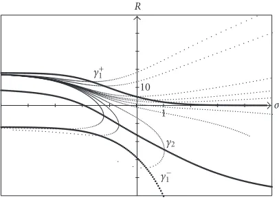
[image:14.468.131.334.68.215.2]σ
Figure 3.1. The phase portrait for system (3.6).
Therefore, taking into account the signs of the right-hand sidesF1andF2, we obtain the phase portrait shown inFigure 3.1.
Now, it is evident the existence of a separatrix which goes fromσ−=ρ0τ/ρ1,R−=e21/ρ0 (forτ→ −∞) toσ+=τ,R+=0 (forτ→ ∞) lying under the isoclineγ+1. This implies the following statement.
Theorem3.1. There exists the separatrix for system (3.6) which coincides with the “points” σ−,R−andσ+,R+. This separatrix can be specified by the scattering-type conditions
σ
τ −→1, R−→0 forτ−→+∞. (3.19) It seems that a similar statement is true in the general case of arbitraryρ1andρ2. In any case, taking into account the limiting values of the convolutions, after cumbersome calculations, it is possible to find the limiting values of the functions
σ−=τ√ρ1ρ2ρ0 , R−=e1e2ρ0 , V+=0 asτ−→ −∞,
σ+=τ, R+=0, V−=0 asτ−→+∞.
(3.20)
4. Calculations of the phase corrections
After solving problem (3.4), (3.5), we can find the phase correctionsϕi1. Using again the
formulas (2.25), we can rewrite (2.40), (2.41) in the following form:
ψ0t d dτ
τϕi1
=G1+ρiui+ (−1)i+1ψ0tL0
ei+R −
ϕi0t def
= fi(U), (4.1)
wherei=1, 2, andU=(σ,R,V).
Now, we readily derive the desired formulas as follows:
ϕi1(τ)=ψ0t1 1τ τ
0 fi(U)dτ
Smoothness ofUimplies the boundedness of fiat the pointτ=0. Thus,ϕi1are bounded at this point. Next, since
G1,L0,R−→0 asτ−→+∞, ϕi0t= ρiui
ei , i=1, 2, (4.3)
the functions fivanish sufficiently rapidly asτ→ ∞. This guarantees the convergence of
the integral in the right-hand sides of (4.2) asτ→ ∞. Hence,
ϕi1(τ)−→0 asτ−→+∞, (4.4)
which confirms the firsta prioriassumption in (2.7). Furthermore,
fi(τ)=ρ
∗u∗−ρ
iui
ρ∗−ρi −ϕi0t+ᏻ
τ2eγτ asτ−→+∞, (4.5)
where we use the notation (2.48) andr=R−,v=V−sinceB11→1,i=2 fori=1, and i=1 fori=2, andγis a number defined by the choice of the regularizationω.
Thus, the integral diverges. By using L’Hospital rule, it is easy to find the limiting value ofϕi1as follows:
ϕi1= 1 ψ0t
ρ∗u∗−ρiui ρ∗−ρi −
ϕi0t
, i=1, 2. (4.6)
This satisfies the firsta prioriassumption in (2.13). Moreover, formulas (4.6) allow to calculate the limiting phasesφi=limτ→−∞φi. Indeed, using the Taylor expansion at the
time instantt=t∗and taking into account equality (2.30), we derive φidef=ϕi0+ψ0(t)ϕi1=x∗+
ϕi0t+ψ0tϕi1
t−t∗
=x∗+ρ∗u∗−ρiui ρ∗−ρi
t−t∗, i=1, 2.
(4.7)
Obviously, these phases satisfy the first Rankine-Hugoniot conditions (2.49).
5. Conclusion
Acknowledgment
The research was supported by SEP-CONACYT under Grant 41421 F and by CONACYT under Grant 43208 (Mexico).
References
[1] A. Bressan,Hyperbolic systems of conservation laws in one space dimension, Proceedings of the International Congress of Mathematicians, vol. I (Beijing, 2002), Higher Education Press, Beijing, 2002, pp. 159–178.
[2] C. M. Dafermos,Hyperbolic Conservation Laws in Continuum Physics, Grundlehren der math-ematischen Wissenschaften, vol. 325, Springer, Berlin, 2000.
[3] V. G. Danilov,Generalized solutions describing singularity interaction, Int. J. Math. Math. Sci.29 (2002), no. 8, 481–494.
[4] V. G. Danilov, G. A. Omel’yanov, and V. M. Shelkovich,Weak asymptotics method and inter-action of nonlinear waves, Asymptotic Methods for Wave and Quantum Problems, Amer. Math. Soc. Transl. Ser. 2, vol. 208, American Mathematical Society, Rhode Island, 2003, pp. 33–163.
[5] V. G. Danilov and V. M. Shelkovich,Propagation and interaction of shock waves of quasilinear equation, Nonlinear Stud.8(2001), no. 1, 135–169.
[6] ,Delta-shock wave type solution of hyperbolic systems of conservation laws, Quart. Appl. Math.63(2005), no. 3, 401–427.
[7] D. A. Kulagin and G. A. Omel’yanov,Asymptotics of kink-kink interaction for equations of sine-Gordon type, Mat. Zametki75(2004), no. 4, 603–607 (Russian), translated in Math. Notes 75(2004), no. 3-4, 563–567.
[8] P. G. LeFloch,Hyperbolic Systems of Conservation Laws. The Theory of Classical and Nonclassical Shock Waves, Lectures in Mathematics ETH Z¨urich, Birkh¨auser, Basel, 2002.
[9] B. L. Rozhdestvenski˘ı and N. N. Yanenko,Systems of Quasilinear Equations and Their Applica-tions to Gas Dynamics, 2nd ed., Nauka, Moscow, 1978, English translation, American Math-ematical Society, Rhode Island, 1983.
[10] G. B. Whitham,Linear and Nonlinear Waves, Pure and Applied Mathematics, John Wiley & Sons, New York, 1974.
M. G. Garc´ıa-Alvarado: Departamento de Matem´aticas, Universidad de Sonora, 83000 Sonora, Mexico
E-mail address:[email protected]
R. Flores-Espinoza: Departamento de Matem´aticas, Universidad de Sonora, 83000 Sonora, Mexico
E-mail address:[email protected]
G. A. Omel’yanov: Departamento de Matem´aticas, Universidad de Sonora, 83000 Sonora, Mexico