PROBLEM FOR ESTIMATING HEAT SOURCE
A. SHIDFAR, A. ZAKERI, AND A. NEISIReceived 28 May 2002 and in revised form 9 May 2005
This note considers the problem of estimating unknown time-varying strength of the temporal-dependent heat source, from measurements of the temperature inside the square domain, when the prior knowledge of the source functions is not available. This problem is an inverse heat conduction problem. In this process, the direct problem will be solved by using the heat fundamental solution. Then a sequential algorithm is devel-oped to solve a Volterra integral equation, which has been produced by using unknown source term and overposed data conditions. This algorithm is based on the piecewise lin-ear continuous functions. The performance of the present technique of inverse analysis is evaluated, by means of several numerical experiments, and is found to be very accurate as well as efficient.
1. Introduction
An inverse heat conduction problem is concerned with the determination of the un-known source term, from the knowledge of directly measurable quantities such as tem-perature inside the domain. Obviously, the solution of these inverse problems is not straightforward due to their ill-posedness, and it requires special numerical techniques to stabilize the result of calculations [1,8,9,10,11].
For this purpose, the least-squares method will be modified by the addition of reg-ularization terms that impose additional restrictions on admissible solutions. This idea has been provided by ¨Ozisik, Orlande, Park, Chung, and Jung in [5,6,12]. In [5,7], a se-quential algorithm where initial a priori estimation is continuously updated based on the current experimental measurements is used. In this process, the triangular shape func-tions with the Karhunen-Lo`eve decomposition method has been applied. The sensitivity and adjoint problems are described in [5,12].
We use the heat fundamental solution for direct problem, and then by choosing the strength of the form of a finite series of shape functions with unknown constant coeffi-cient and applying a linear least-squares method, the term heat source will be estimated. A numerical experiment is given in the final section of this note.
Copyright©2005 Hindawi Publishing Corporation
2. Mathematical formulation
Let D= {(x,y)|0< x < L, 0< y < L} be a square domain in R2. To illustrate the
methodology for determining unknown location and strength of a heat source by the se-quential and Tikhonov regularization methods, the governing equation for the heat con-dition induced by a time-varying heat source,g(t) located at (x∗,y∗)∈Din the square D, the Neuman boundary conditions, and a temperature distribution at zero time are in the form
ρc∂tT(x,y,t)=k∇2T(x,y,t) +g(t)δ(x−x∗,y−y∗), (x,y)∈D, 0< t < tf, (2.1) T(x,y, 0)=T0(x,y), (x,y)∈D∪∂D, (2.2)
∂xT(0,y,t)=0, 0≤y≤L, 0≤t≤tf, (2.3) ∂xT(L,y,t)=P(y,t), 0≤y≤L, 0≤t≤tf, (2.4) ∂yT(x, 0,t)=0, 0≤x≤L, 0≤t≤tf, (2.5) ∂yT(x,L,t)=Q(x,t), 0≤x≤L, 0≤t≤tf, (2.6)
whereδ(·) is the Dirac delta function,tf,k,ρ, andcare constant numbers, and are called final time, thermal conductivity, density, and specific heat of the material, respectively. We will assume through out the note thatP,Q, andT0are piecewise continuous functions.
By putting
T(x,y,t)=u(x,y,t) +v(x,y,t), (2.7)
then, the problem (2.1)–(2.6) may be converted to
ρc∂tu(x,y,t)=k∇2u(x,y,t), (x,y)∈D, 0< t < tf, u(x,y, 0)=T0(x,y), (x,y)∈D∪∂D,
∂xu(0,y,t)=0, 0≤y≤L, 0≤t≤tf, ∂xu(L,y,t)=P(y,t), 0≤y≤L, 0≤t≤tf,
∂yu(x, 0,t)=0, 0≤x≤L, 0≤t≤tf, ∂yu(x,L,t)=Q(x,t), 0≤x≤L, 0≤t≤tf,
(2.8)
ρc∂tv(x,y,t)=k∇2v(x,y,t) +g(t)δ(x−x∗,y−y∗), (x,y)∈D, 0< t < tf, v(x,y, 0)=0, (x,y)∈D∪∂D,
∂nv(x,y,t)=0, (x,y)∈∂D, 0≤t≤tf,
(2.9)
Obviously, the problem (2.8) is a direct problem, it has a unique solution in the form [2]
u(x,y,t)=
DN(x,ξ,y,η,t)T0(ξ,η)dξ dη + 2
L
0
t
0θ(x−L,y−η,t−τ)P(η,τ)dτ dη
+ 2 L
0
t
0θ(x−ξ,y−L,t−τ)Q(η,τ)dτ dξ,
(2.10)
where
N(x,ξ,y,η,t)=θ(x−ξ,y−η,t) +θ(x+ξ,y+η,t),
θ(x,y,t)= ∞
m=−∞ ∞
n=−∞
K(x+ 2m,y+ 2n,t) (2.11)
is theθ-function in two-dimensional space and
K(x,y,t)= k
4πρctexp
−kx2+y2
4ρct
(2.12)
that may be derived from
K(x,t)=√1
4πtexp −x2
4t
, (2.13)
the fundamental solution of the one-dimensional heat equation. Now, ifg(t) is a known bounded function inL2(0,t
f), then the problem (2.9) is a direct heat conduction problem. The unique solution of this problem may be represented by
v(x,y,t)= L
0
L
0
t
0N(x,ξ,y,η,t−τ)g(τ)δ(ξ−x
∗,η−y∗)dτ dξ dη
= t
0N(x,x
∗,y,y∗,t−τ)g(τ)dτ.
(2.14)
Now, if (2.1)–(2.6) is a problem with a known source term and unknown time-depending strength g(t), then it is an inverse problem. For finding an unknown functiong(t) in (2.14), we use the overposed data condition in the form
Tx1,y1,t
=Y(t), 0≤t≤tf, (2.15)
and using (2.10) and (2.14), we derive a Volterra integral equation in the form
f(t)=Y(t)−ux1,y1,t
=
t
0N
x1,x∗,y1,y∗,t−τ
g(τ)dτ, 0≤t≤tf. (2.16)
Ifg(t)∈L2(0,t
f), then the problem (2.16) has unique solution [2].
Because problem (2.16) is an ill-posed problem, the regularization method must be utilized in order to obtain a useful approximation to the desired solution.
In the next section, the sequential algorithm with triangular shape functions will be used for estimating the solution of (2.16). In this algorithm, the shape functions are used.
3. Numerical scheme
In this section, we suppose thatg(t) in the problem (2.1)–(2.6) is an unknown function. Then, the unknown functiong(t) will be estimated by using the temperature histories taken at (x1,y1)∈Dover the interval of time [0,tf]. For this purpose, we employ a nu-merical method to solve the first-kind Volterra integral equation (2.16), with convolution kernelN, on [0,tf].
LetM=1, 2,. . .be an arbitrary integer constant number,∆t=tf/M, andti=i∆tfor anyi=0,. . .,M. Then the approximate solutiong∗(t) is chosen in the form
g∗(t)=
M
m=1
gm∗Φm(t), (3.1)
whereΦm(t) is themth base function defined by
Φm(t)=
t−tm−1
tm−tm−1, tm−1≤t≤tm,
tm+1−t
tm+1−tm, tm≤t≤tm+1,
0 elsewhere.
(3.2)
We note that{Φm(t)}M
m=1is the orthonormal set in C[0,tf]. The goal of this section is to show that the approximate vectorg∗=(g1∗,. . .,gM∗)T defined by the discrete sequential Tikhonov regularization algorithm is a suitable approximation forf=(f(t1),. . .,f(tM))T for appropriate choices oft1,. . .,tM∈[0,tf], andM∈N, instead ofg=(g1,. . .,gM)T. Such parameter estimation problem is solved by the minimization of the ordinary least-squares method.
By putting (3.1) in (2.16), at successive timet=ti,i=1,. . .,M, we obtain
f(t1)=
M
m=1
gm∗ t1
0 N
x1,x∗,y1,y∗,t1−τ
φm(τ)dτ
=g1∗
t1
0 N
x1,x∗,y1,y∗,t1−τ
φ1(τ)dτ,
f(ti)=
M
m=1
gm∗ ti
0 N
x1,x∗,y1,y∗,ti−τ
φm(τ)dτ
=
i−1
m=1
gm∗ tm+1
tm−1
Nx1,x∗,y1,y∗,ti−τφm(τ)dτ
+gi∗ ti
ti−1
Nx1,x∗,y1,y∗,ti−τφi(τ)dτ
= i−
1
m=1
gm∗ t2
0 N
x1,x∗,y1,y∗,ti−m+1−τ
φ1(τ)dτ
+gi∗ t1
0 N
x1,x∗,y1,y∗,t1−τ
φ1(τ)dτ
=
i−1
m=1
gm∗ai−m+1+gi∗a1, i=2,. . .,M,
(3.4)
where
a1=
t1
0 N
x1,x∗,y1,y∗,t1−τ
φ1(τ)dτ, (3.5)
ai= t2
0 N
x1,x∗,y1,y∗,ti−τ
φ1(τ)dτ, i=2,. . .,M. (3.6)
Now, consider the system of equations
Ag∗=f, (3.7)
which is obtained by (3.1)–(3.6), such thatA∈RM×M is a lower-triangular Toeplitz ma-trix given by
A=
a1 0 ··· 0
a2 a1 ··· 0
..
. ... . .. ... aM aM−1 ··· a1
, (3.8)
and thatai>0, for alli.
Therefore, we can drive a convergence and stable solution to (3.7) by the fast algo-rithm for the implementation of sequential Tikhonov regularization method described by Lamm and Eld´en in [3,4].
In order to find the solution of the system equations (3.7), we define
J(g∗)=
M m=1 m i=1
am−i+1gi∗−fi 2
+α m
i=1
m−i+1gi∗
2
whereα >0 is a given regularization parameter and
L=
1 0 ··· 0
2 1 ··· 0
..
. ... . .. ...
M M−1 ··· 1
(3.10)
is a lower-triangular Toeplitz matrix instead ofIin the sequential Tikhonov regularization algorithm. In the end of this section, the effective choice ofLwill be expressed. The least-squares procedure for the estimation ofg∗applies for the minimization ofJ(g∗) in (3.9). J(g∗) will be minimized by differentiating with respect to unknown parameterg∗ for any=1,. . .,M, and then setting the resulting expression equal to zero. Consequently by using [4], we can obtain the unknown vectorg∗as in the following process. Assuming thatg1∗,. . .,gi−∗1have already been found, then by putting
h(1)=f1,. . .,fr
, h(i)=h(i)
1 ,. . .,h(ri)
, i≥2, (3.11)
with
h(pi)= fi+p−1−
i−1
j=1
ai+p−jg∗j, p=1,. . .,r < M, (3.12)
we determinegi∗by finding the vectorβ=(β1,. . .,βr) from the minimization ofJ(β) in
the form
J(β)=
r
m=1
m
k=1
am−k+1βk−fk 2
+α m
k=1
m−k+1βk 2
. (3.13)
Substitutingg∗in (3.1),g(t) will be approximated for 0< t≤tf.
Finally, in this section by using [3,4], we express the following theorems for conver-gence and stability of the above procedure.
Theorem3.1. Assume that r=1, 2,. . .is a fixed integer and letg∈C[0,tf], whereg is the solution of (2.16) on [0,tf]using precise data f. In addition, assume that for δ >0, the perturbed data fδ(t)satisfies in fδ(t)= f(t) +d(t),t∈[0,t
f], with|d(t)|< δont∈ [0,tf]. Then ifα=α(t)is selected such thatα=αˆ∆t2withα >ˆ 0and∆t=∆t(δ)satisfies ∆t(δ)=τ√δwith a constant numberτ >0, it follows that asδ→0,∆t(δ)→0,α(∆t)→0, and
g−g
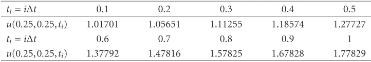
Table 4.1. Overposed exact matching data foruintiand location (0.25, 0.25).
ti=i∆t 0.1 0.2 0.3 0.4 0.5
u(0.25, 0.25,ti) 1.01701 1.05651 1.11255 1.18574 1.27727
ti=i∆t 0.6 0.7 0.8 0.9 1
u(0.25, 0.25,ti) 1.37792 1.47816 1.57825 1.67828 1.77829
asδ→0, whereC¯(r)is a fixed positive constant andg=(g1,. . .,gM)is the solution of the problem (3.3)–(3.4) based on using perturbed data fδ(t).
Proof. The proof of this theorem is given by Lamm and Eld´en in [3,4], when the so-lution of the sequential Tikhonov regularization problem for approximations based on piecewise constant functions, rectangular quadrature, or midpoint quadrature. By using the mean-value theorem for integrals in (3.3) and (3.4) in the form
a1=
t1
0 N
x1,x∗,y1,y∗,t1−τ
φ1(τ)dτ
=φ1(ζ)
t1
0 N
x1,x∗,y1,y∗,t1−τ
dτ, for 0< ζ < t1,
ai= t2
0 N
x1,x∗,y1,y∗,ti−τ
φ1(τ)dτ
=φ1(ρ)
t2
0 N
x1,x∗,y1,y∗,ti−τ
dτ, for 0<ρ< t2,i=2,. . .,M,
(3.15)
and applying the similar method to the processes of their prove, the proof of the above
theorem is investigated.
In the next section, a numerical sample is given and the performance of the present technique of inverse analysis is evaluated.
4. Numerical example
For the inverse problem (2.1)–(2.6), we use the inverse technique for (2.1) defined on the square D= {(x,y)|0< x <1, 0< y <1}, 0< t≤1, andk=ρ=c=1 in following example.
Example 4.1. Consider the inverse heat conduction problem
∂tT(x,y,t)= ∇2T(x,y,t) +g(t)δ(x−0.5,y−0.5), (x,y)∈D, 0< t <1, T(x,y, 0)=1, (x,y)∈D∪∂D,
∂nT(x,y,t)=0, (x,y)∈∂D, 0≤t≤1.
(4.1)
0.2 0.4 0.6 0.8 1 0.2
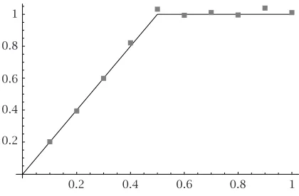
[image:8.468.128.338.67.205.2]0.4 0.6 0.8 1
Figure 4.1. Exact and estimated solution forg(t).
The exact solution functionsu(x,y,t) andg(t) are in the form
u(x,y,t)= ∞
m=1
2 cos(0.5mπ) cos(mπx) t
0g(τ) exp
−m2π2(t−τ)dτ
+ ∞
n=1
2 cos(0.5mπ) cos(nπ y) t
0g(τ) exp
−n2π2(t−τ)dτ
+ ∞
m=1
∞
n=1
4 cos(0.5mπ) cos(0.5nπ) cos(mπx) cos(nπ y)
× t
0exp
−m2+n2π2(t−τ)g(τ)dτ
+ t
0g(τ)dτ+ 1,
g(t)=
2t, 0≤t≤0.5, 1, 0.5≤t≤1.
(4.2)
An approximate solution functiong(t) has been derived in the discrete time by solving the integral equation (2.16) by the sequential Tikhonov regularization algorithm based on triangular functions in (3.1). In this process, we assumed thatα=10−3 andLis the
identity matrixI. The exact and approximate solution functiong(t) withFigure 4.1 fol-lows.
References
[1] G. Alessandrini and V. Isakov,Analyticity and uniqueness for the inverse conductivity problem, Rend. Istit. Mat. Univ. Trieste28(1996), no. 1-2, 351–369.
[2] J. R. Cannon,The One-Dimensional Heat Equation, Encyclopedia of Mathematics and Its Ap-plications, vol. 23, Addison-Wesley, Massachusetts, 1984.
[3] L. Eld´en,An efficient algorithm for the regularization of ill-conditioned least squares problems
with triangular Toeplitz matrix, SIAM J. Sci. Statist. Comput.5(1984), no. 1, 229–236.
[4] P. K. Lamm and L. Eld´en,Numerical solution of first-kind Volterra equations by sequential
[5] M. N. ¨Ozisik and H. R. B. Orlande,Inverse Heat Transfer, Fundamentals and Applications, Taylor and Francis, New York, 2000.
[6] H. M. Park and O. Y. Chung,An inverse natural convection problem of estimating the strength of
a heat source, Int. J. Heat Mass Transfer42(1999), no. 23, 4259–4273.
[7] H. M. Park and W. S. Jung,A recursive algorithm for multidimensional inverse heat conduction
problems by means of mode reduction, Chem. Eng. Sci.55(2000), no. 21, 5115–5124.
[8] A. Shidfar and R. Pourgholi,Application of finite difference method to analysis an ill-posed prob-lem, to appear in Appl. Math. Comput.
[9] A. Shidfar and A. Zakeri,Asymptotic solution for an inverse parabolic problem, Math. Balkanica (N.S.)18(2004), no. 3-4, 475–483.
[10] ,A numerical technique for backward inverse heat conduction problems in one
dimen-sional space, to appear in Appl. Math. Comput.
[11] A. N. Tikhonov and V. Y. Arsenin,Solutions of Ill-Posed Problems, Scripta Series in Mathematics, V. H. Winston & Sons, District of Columbia, 1977.
[12] C.-Y. Yang,Solving the two-dimensional inverse heat source problem through the linear
least-squares error method, Int. J. Heat Mass Transfer41(1998), no. 2, 393–398.
A. Shidfar: Department of Mathematics, Iran University of Science and Technology, Narmak, Tehran 16844, Iran
E-mail address:[email protected]
A. Zakeri: Department of Mathematics, Iran University of Science and Technology, Narmak, Tehran 16844, Iran
E-mail address:a [email protected]
A. Neisi: Department of Statistics, Faculty of Economics, Allameh Tabatabaie University, Dr. Be-heshti Avenue, Tehran 15136-15411, Iran