Validating Solid Wall Insulation Retrofits with In Use Data

Citation:

Hardy, ALR and Glew, D and Fletcher, M and Gorse, C (2018) Validating Solid Wall Insulation

Retrofits with In-Use Data.

Energy and Buildings, 165.

pp.

200-205.

ISSN 0378-7788 DOI:

https://doi.org/10.1016/j.enbuild.2018.01.053

Link to Leeds Beckett Repository record:

http://eprints.leedsbeckett.ac.uk/4697/

Document Version:

Article

Creative Commons: Attribution-Noncommercial-No Derivative Works 4.0

The aim of the Leeds Beckett Repository is to provide open access to our research, as required by

funder policies and permitted by publishers and copyright law.

The Leeds Beckett repository holds a wide range of publications, each of which has been

checked for copyright and the relevant embargo period has been applied by the Research Services

team.

We operate on a standard take-down policy.

If you are the author or publisher of an output

and you would like it removed from the repository, please

contact us

and we will investigate on a

case-by-case basis.

Validating Solid Wall Insulation Retrofits with In-Use Data

A. Hardya,∗_{, D.Glew}a_{, C. Gorse}a_{, M. Fletcher}a

a_{Leeds Beckett University, Leeds, LS2 9EN}

Abstract

Improving the energy efficiency of the UK housing stock is important both to meet carbon emission reduction targets and to reduce fuel poverty. For this reason, domestic properties are frequently retrofitted with energy saving measures. This study looks at how the energy consumption, thermal properties and internal temperature of 14 dwellings change as a result of a solid wall insulation (SWI) retrofit. A decrease in heat transfer coefficient of 11+6₋₇% was calculated for 2 dwellings, which is slightly lower than the previously modelled value of 18%. However, many houses displayed evidence that the full benefit of SWI was not being realised as, for example, energy savings were offset with increases in internal temperature. Future retrofit schemes should therefore consider supplementing the changes in fabric with increased guidance for the occupant.

Keywords: Solid Wall Insulation, Retrofits, In-Use data

1. Introduction

In 2015, the domestic sector accounted for 29% of UK total energy consumption [1] and of this percentage, space heating can account for around 60% [2]. The large amount of energy expended on domestic heating means that reduc-5

tion strategies are vital if the UK government is to reach is target of cutting greenhouse gas emissions by 80% by the year 2050 [3]. Two of the simplest ways to reduce emissions from domestic heating are to ensure that houses are heated efficiently and to ensure they retain that heat well. Legis-10

lation is currently in place to work towards this, with the 1995 edition of the 1991 UK Building Regulations being the first that required step changes in energy efficiency re-quirements of new homes [4]. However, the English Hous-ing Survey reports that over 80% of homes were built prior 15

to this legislation coming into force and these homes are therefore expected to have generally poorer thermal per-formance [5]. This means that large scale retrofitting is crucial for increasing the efficiency of houses [6], and it has also been demonstrated that wider socio-economic health 20

and community wide benefits can be achieved via retrofit policy [7, 8, 9].

Recent retrofit efforts including the Carbon Emissions Reduction Target (CERT), Renewable Heat Incentive (RHI), Community Energy Saving Programme (CESP) and the 25

Energy Companion Obligation (ECO) have been relatively effective, as reflected in the fact that dwellings with A-C Energy Performance Certificate (EPC) ratings have risen from just 5% in 2005 to 28% in 2015 [5]. This also im-plies, however, that there is still a substantial way to go 30

∗_{Corresponding author}

Email address: [email protected](A. Hardy)

and it has been suggested that in order to meet the 5th UK Carbon Budget, the domestic sector is expected to cut emissions by a further 22% between 2015 and 2020 [10].

There are several options available when retrofitting a dwelling that can focus on the fabric or the services in 35

the home. Of the 2 million measures installed via ECO, 38% were cavity wall insulation (CWI), 26% loft insulation and 21% boiler upgrades [11]. Government statistics on annualised gas data from a large number of homes show that these measures result in a saving of 8.4%, 2.1% and 40

8.3% respectively on average household fuel bills[12]. As a result, these three measures are often deemed to have the most carbon savings.

The benefits of solid wall insulation (SWI) are less well studied, with this lack of information due, at least in part, 45

to the relatively low installation rate of SWI. This is a significant oversight since 34% of the UK housing stock is estimated to have solid walls, 98% of which remain unin-sulated [13]. A summary of literature on the potential savings from SWI has been published by the BRE [13], 50

and individual case studies often reveal that SWI can re-sult in higher savings than CWI - upwards of 60% [14] or even 80% when part of a deep renovation [15]. However, assessment methods used to validate the effectiveness of retrofits on small numbers of dwellings, as in the case of 55

SWI, inherently have low statistical power and high uncer-tainty. Conversely, savings for conventional measures are derived from samples of tens of thousands of homes [12].

SWI may be applied as internal wall instulation (IWI) or external wall insulation (EWI), with installation ap-60

es-timates for the effect of EWI suggest an 18% reduction 65

in heat loss from the property [16]. However, owing to a lack of empirical data at the time, this figure was derived from building energy models which, in general, have been shown to overestimate the affect of improvements [7, 17]. The gap between the predicted and measured performance 70

is due to a combination of factors, including the model’s inability to fully incorporate all physical affects, its failure to reflect real-world insulation procedures and its reliance on standardised assumptions around occupant behaviour [18]. In-use factors are often used in an attempt to account 75

for the occupant behaviour, but the uncertainty surround-ing these adjustments is still high [13]

Gathering more data on SWI improvements is there-fore of great importance to provide more certainty around costs and benefits of this measure, and will potentially al-80

low more effective policy to be written. Similarly, it is important to develop robust assessment methods in order to understand how savings achieved from particular SWI projects compare to savings from more common methods such as cavity wall insulation. This study aims to achieve 85

these two goals by presenting the results from long-term measurement of energy consumption and temperature in 14 solid wall dwellings in which SWI retrofits were under-taken. The project findings will provide insight into the 6.3 million solid wall dwellings in the UK that may in the 90

future have a retrofit [5]. Given the substantial remaining potential and the fact that there will be minimum quotas for SWI in the Help to Heat policy [19], understanding the real improvements achieved by SWI installation is of particular importance in the UK and in other countries ex-95

periencing similar domestic energy policy challenges with large proportions of solid wall dwellings in their housing stock.

2. Observations

Retrofit installers, Registered Social Landlords (RSLs) 100

and Local Authorities (LAs) across the North of Eng-land who were taking part in government funded domes-tic retrofit programmes were invited to take part in this research. Securing samples proved challenging, but conve-nience sampling and snow ball sampling resulted in over 105

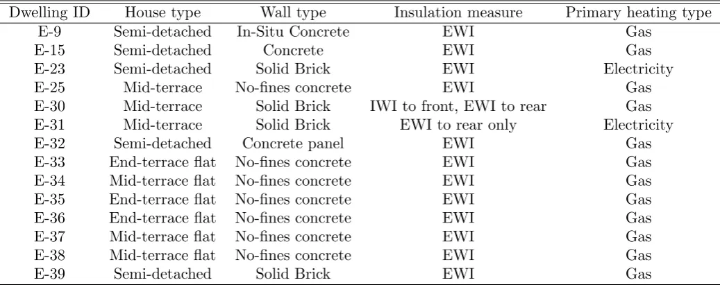
1,000 properties being invited to take part in the project from which 45 properties accepted. Of these 45 homes, 14 had retrofits suitable for inclusion in the study and took place within the research project time-scale. Within the sample of 14 properties, 10 had solid concrete walls (e.g. 110

pre fab or no-fines) built between 1950 and 1970 and 4 had solid brick walls built pre 1910 (see table 1). These property ages are representative of a substantial propor-tion of solid walls dwellings in the UK housing stock, as 17% of homes in the UK were built before 1910, and 28% 115

were built between 1945 and 1974 [20]. However, there is an over-representation of concrete walls in this sample compared to the UK housing stock, as approximately 86%

Figure 1: The number of days of data available either side of the retrofit. Some houses have minimal data taken before the retrofit took place.

Dwelling ID

E-09

E-15

E-23

E-25

E-30

E-31

E-32

E-33

E-34

E-35

E-36

E-37

E-38

E-39

400 200 0 200 400 600

Number of days of monitoring Before retrofit After retrofit

of solid walls in the UK are masonry and only 14% are concrete [21].

120

In-use data was captured in each dwelling at half hourly intervals with Orsis sensors and included, where possible, gas (m3_{), electricity (kWh), internal temperature (}◦_{C) for}

both upstairs and downstairs, and external temperature (◦C). During the course of these measurements, SWI was 125

installed in all of the properties. The installations were taking place independently to the research project and al-though the occupants were informed of the project, the installers were not. It is therefore anticipated the work-manship of the SWI was representative of a standard in-130

stallation processes.

The observations and retrofits took place between 2013 and 2016 though the actual monitoring duration at each home differed according to when they had their monitor-ing installed and if there were delays in the retrofit occur-135

ring. How the measured data was distributed pre and post retrofit is shown in Figure 1.

Table 1: Summary of dwelling retrofits

Dwelling ID

House type

Wall type

Insulation measure

Primary heating type

E-9

Semi-detached

In-Situ Concrete

EWI

Gas

E-15

Semi-detached

Concrete

EWI

Gas

E-23

Semi-detached

Solid Brick

EWI

Electricity

E-25

Mid-terrace

No-fines concrete

EWI

Gas

E-30

Mid-terrace

Solid Brick

IWI to front, EWI to rear

Gas

E-31

Mid-terrace

Solid Brick

EWI to rear only

Electricity

E-32

Semi-detached

Concrete panel

EWI

Gas

E-33

End-terrace flat

No-fines concrete

EWI

Gas

E-34

Mid-terrace flat

No-fines concrete

EWI

Gas

E-35

End-terrace flat

No-fines concrete

EWI

Gas

E-36

End-terrace flat

No-fines concrete

EWI

Gas

E-37

Mid-terrace flat

No-fines concrete

EWI

Gas

E-38

Mid-terrace flat

No-fines concrete

EWI

Gas

E-39

Semi-detached

Solid Brick

EWI

Gas

3. Data pre-processing

Before the data could be analysed, it was first inspected to identify any possible errors. Given that the dataset in-140

cluded approximately eight million data-points, this pre-processing was largely automated and included the follow-ing producers;

First, it was noted that the raw data included many periods of “drop-out”, in which no data was recorded or 145

sent to the loggers. Data which suffered from these drop-outs was padded with timestamps containing NA values during the drop-out, so that each day contained the same number of data points for each sensor.

The data were further inspected for any error codes 150

sent by the loggers themselves. For the sensors used, the error code corresponded to a reading of -2. As the min-imum genuine value that the gas and electricity sensors could record was 0, any value of -2 in the electricity and gas data was certainly an error and was therefore replaced with 155

an NA value. For the temperature sensors, however, it was possible that genuine values of -2 may have been recorded. Genuine values of -2 where therefore distinguished from error codes by searching for rapid temperature changes to -2 and back. Data points fitting this description were 160

identified using methods of outlier detection in time series [22, 23], and flagged as potential errors.

Finally, it was observed that several periods of the elec-tricity and gas data contained “flatlines” - periods of time over which the same non-zero value is recorded. The cause 165

of these flatlines is not clear, but the resolution of the elec-tricity and gas sensors (1kWh and 0.001m3_{, respectively) is}

high enough that such constant readings over a prolonged period are unlikely to be genuine. Shorter periods of flat readings are potentially genuine, however, so we chose a 170

dividing line of 3 hours to distinguish flatline errors. A rolling 3-hour window was applied to the data and any

periods for which the readings were finite and constant were marked as a likely flatline errors.

The majority of the data did not raise any flags to 175

indicate potential errors. Only ∼0.005 % of data points were identified as potential anomalies, and this low number allowed those error flags to be checked in person. Any confirmed errors were replaced with NA values.

4. Analysis

180

4.1. Changes in Electricity and Gas use

The first effect of the retrofit to be studied was that of any changes in the household electricity and gas con-sumption. Before this analysis was carried out, however, the consumption values were first weather corrected. A 185

weather correction is often applied as, in addition to build-ing improvements, weather can affect the energy consump-tion of a household. For example, a period of relatively warm weather after retrofit may result in a reduction in utility use due to the lower heating demand. A weather 190

correction adjusts the utility consumption values in an at-tempt to remove the weather component and allow the affect of the retrofit to be isolated. The weather correc-tion was achieved by multiplying the heating utility con-sumption values by the proportional difference in average 195

heating degree day (HDD) between the periods of interest. One HDD was calculated from equation 1 [24].

HDD=

(

0, fortext>15.5

15.5−text, fortext≤15.5

(1)

wheretext is the average external temperature of the day.

For some houses, the difference in HDD’s was sizeable, with a maximum of a 23% increase in the average HDD 200

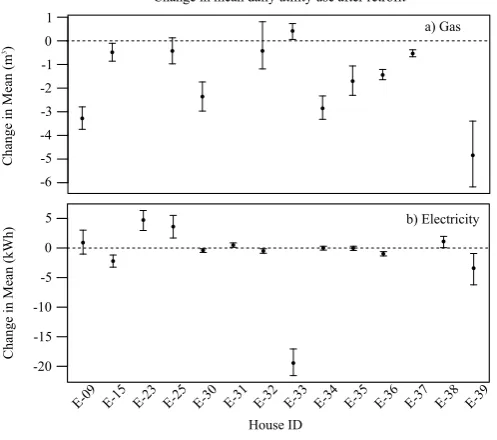
Figure 2: Comparison of the distribution means for gas (top) and electricity (bottom) before and after retrofit. A negative value for a change in the mean suggests a decrease in the use of that utility.

a) Gas

b) Electricity Change in mean daily utility use after retrofit

House ID

Change in Mean (kW

h)

Change in Mean (m

3) 1 0 -1 -2 -3 -4 -5 -6

5

0

-5

-10

-15

-20

E-09 E-15 E-23 E-25 E-30 E-31 E-32 E-33 E-34 E-35 E-36 E-37 E-38 E-39

The total daily electricity and gas consumption was then calculated for days in which heating was likely being used, defined as between the 1st of November and the of 1st of April. These months were chosen as they are typ-205

ically the coldest 5 months of the year [25]. These daily consumption values were split into distributions before and after retrofit. In the cases where exact dates of the start or finish of the retrofit were not available, a one month window around the approximate date was used.

210

The distributions of gas and electricity consumption were non-normal, and a comparison of the two distribu-tions was therefore achieved using a wilcoxon rank sum test. This test determines if there is a statistical difference in the mean of the two distributions, and the results of 215

this test are plotted in figure 4.1. A negative value for the change in mean corresponds to a reduction in daily mean utility use, and any values whose error bars overlap 0 have no significant difference in their means at the 95% confi-dence level. Several houses are missing from these graphs 220

due to data not being available. Houses E-23 and E-31 are missing gas data, but this is because they use electricity for heating. House E-38 does use gas, but a sensor fault caused the lack of gas data. Likewise, house E-37 uses electricity, but a sensor fault caused the lack of electricity 225

data.

It is apparent from these data that 8 of the 14 houses display a significant decrease in their daily mean gas use. 2 houses have no significant change, and 1 house shows a significant increase in its daily gas use. For electricity, 230

6 of the houses have a significant decrease in their daily use (although the decrease is small in 3 of these cases),

Figure 3: Change in the daily CO2 emission associated with each

properties energy use as a result of retrofit. The data are color coded, where red points denote houses which showed a general in-crease in internal temperature after retrofit, where blue points denote houses which showed a general decrease in internal temperature after retrofit.

House ID

E-09 E-15 E-23 E-25 E-30 E-31 E-32 E-33 E-34 E-35 E-36 E-37 E-38 E-39

Change in Mean (kg)

0

-5

-10

Change in mean daily CO2 emission after retrofit

3 have no significant change, and 4 show a significant in-crease. Combining the data displayed on these two graphs further gives insight into any changes in how a household 235

is heated. In the most obvious example, E-33 reports a slight increase in gas use but a considerable drop in elec-tricity use, suggesting occupants relied heavily on electric heating before the retrofit and now rely more on gas heat to their house.

240

To determine the effect of the retrofit on daily CO2

emission, the values of daily gas and electricity were con-verted to associated values of CO2 emission using UK

government greenhouse gas conversion factors [26]. The results are displayed in figure 4.1. It is apparent from 245

this figure that the increase in gas consumption for E-33 is compensated for by its decrease in electricity use. In-deed, the only houses which show an increase in associated daily CO2emission are the two properties which are heated

electrically. The increase in utility use for these proper-250

ties may be a manifestation of the rebound effect [27], in which gains in energy efficiency are offset by increased energy consumption after retrofit causing potential over-heating. Likewise, it may be that they properties were suffering from the prebound effect [28], which describes a 255

situations in which heating systems are under-used prior to retrofit due to their inefficiency. Removing this ineffi-ciency therefore may result in increased use of the heating system. In either case, the rebound and prebound effects are both associated with increased internal temperatures. 260

The internal temperature of the properties was therefore studied to offer further insight.

4.2. Changes in Internal Temperature

The change in mean internal temperature was calcu-lated in the same manner to the electricity and gas data. 265

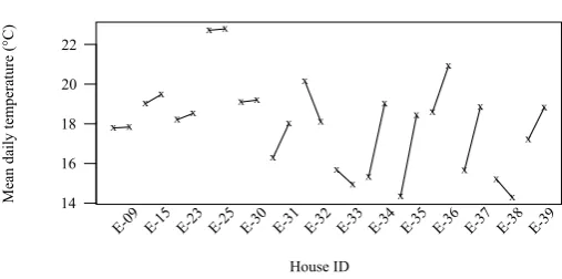
The results are displayed in figure 4. Many of the houses display an increase in internal temperature, suggesting that potential energy savings are at least partially offset by an increase in internal temperature. In five of these cases (E-31, E-34, E-35, E-37, E-39), the internal tem-270

perature was below the suggested value for thermal com-fort of 18◦C[29] before retrofit, and subsequently increased to within the comfortable region. These properties may therefore have been suffering from the prebound effect. E-31 is particularly interesting, as it shows a marginal in-275

crease in energy use after retrofit. Although the retrofit was not successful in reducing energy use, the increased tempearture has likely reduced the risk of ill-health, espe-cially as the pre-retrofit survey data described the house as being particularly cold and damp.

280

E-23 is the other instance in which an increase in util-ity use and associated CO2 emission after retrofit was

re-ported. The increase in internal temperature for E-23 is marginal, and both values are within a comfortable re-gion. The increase in utility consumption for this property 285

might therefore be due to increased occupancy, increased ventilation (with occupants opening more windows), or a combination of the two factors. E-32 is another instance where the data suggests increased ventilation after retrofit. E-32 shows no significant change in associated CO2

emis-290

sion, but a sizeable decrease in internal temperature. It may therefore be that the heating controls are unsuitable or misunderstood, and occupants now combat overheating of the property with open windows.

E-33 and E-38 show a temperature decrease and both 295

values are below the normal ranges for comfort. Financial strain may be the reason for the lack of heating in these cases, and would also explain how such a large decrease in electricity was achieved for house E-33. If so, the retrofit might not be considered a success, as the reduction in CO2

300

emission is partly due to increased fuel-poverty and the retrofit was unable to remedy this.

4.3. Grey-box Modelling

As a result of the rebound and prebound effects men-tioned in section 4.1, reductions in utility use cannot be di-305

rectly related to increases in building fabric performance. For example, a property might have its building fabric improved by 10% but show no reduction in utility use if occupants have chosen to increase the temperature of their property. To determine what the true fabric im-310

provement is, grey-box modelling was therefore performed on the data. Grey-box modelling considers both the data on utility use and temperatures, and combines these with a physical model of the house. This technique has been shown to provide robust models for physical systems [30, 315

31] and, although other methods for the determination of building characteristics exist, other methods often have constraints such as the requirement that no heating be em-ployed throughout the night period [32]. Grey-box mod-elling does not have these constraints, placing it amongst 320

the most versatile methods available when modelling houses

Figure 4: Change in the daily average temperature as a result of retrofit. The first point for each house denotes the mean daily perature before retrofit, and the second point the mean daily tem-perature after retrofit. A positive gradient in the connecting line therefore shows an increase in internal temperature between the time periods. The uncertainties on the points are negligible.

x x x x x x x x x x x x x x x x x x x x x x x x x x x x Mean dail

y temperature (°C

) 22 20 18 16 14 House ID

E-09 E-15 E-23 E-25 E-30 E-31 E-32 E-33 E-34 E-35 E-36 E-37 E-38 E-39

Change in mean daily internal temperature after retrofit

with differing heating patterns. A comparison of the opti-mal building models pre and post retrofit can then be used to trace how successful the retrofit was.

The building model employed treated building com-325

ponents as resistors and capacitors, where the values for thermal resistance and capacitance are the constants to be solved for. The change in internal temperature of the house,dTi, was assumed to follow the relationship

dTi=

1

Ci

[ 1

Ri

(Tw−Ti) +Hp∗Igas]dt+σidωi(t) (2)

whereCithe thermal mass of the heated environment,

330

Ri the resistance of the internal environment, Tw is the

wall temperature, Ti the internal average temperature,

Hp is a constant describing the conversion from gas

con-sumption to heat output, Igas the gas consumption due

to heating,ωi is a standard wiener process, describing the

335

stochastic nature of the temperature changes and σi the

scaling factor for the wiener process.

The wall temperature, Tw was not measured in this

study, but the external temperature was measured. An-other differential equation was therefore set up to describe 340

the wall temperature:

dTw=

1

Cw

[ 1

Ri

(Ti−Tw)+

1

Rwe

(Te−Tw)]dt+σwdωw(t) (3)

where Cw the thermal mass of the wall, Re the

resis-tance between the external environment and the walls and

Te is the external temperature. An RC diagram for the

above system can be seen in figure 5. 345

Figure 5: Physical model applied to the data pre and post retrofit. The values of thermal resistance of the fabric, Riwand Rwe, were of

particular interest.

C

C

R

R

T

T

H

heating season were analysed, as these periods tend to in-clude more heating and greater differences between inter-350

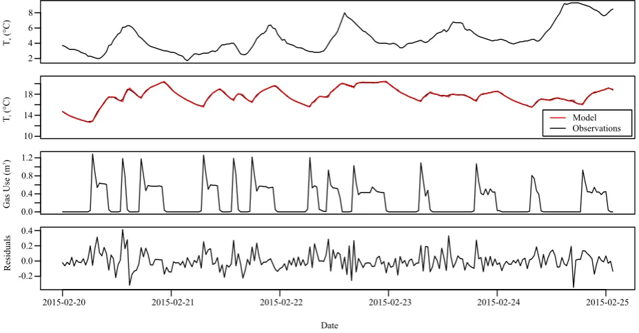
nal and external temperatures which improves model esti-mates [34]. An example of data used in the model fitting procedure is displayed in figure 6. The modelled internal temperature can be seen to approximate the internal tem-perature well and the residuals approximate white noise. 355

A term accounting for solar heating was not included in any models as these data were not available. However, the affect of solar should have a reduced affect within the winter months, and the residuals of the model fits do not indicate a solar term was lacking.

360

The final heat transfer coefficient (HTC) of the house was calculated as the inverse of the sum of the resistances in the model. The error in the HTC was estimated from the Jacobian of the resistance values. The proportional changes in the HTC pre and post retrofit were then calcu-365

lated.

For the majority of the houses, the uncertainty in this proportional change in HTC was very large and, as such, no significant difference could be determined. The large uncertainties are perhaps because the model does not in-370

clude non-linear effects such as wind, nor does it account for physical changes to the building envelope such as the opening of doors and windows. These factors could not be included as no data was available. A lack of data for some houses also contributed to their large uncertainties, as pre-375

vious work has suggested at least 20 days of monitoring is required for accurate grey-box modelling [34], and 2 of the houses did not meet this requirement (see Figure 1.

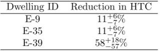
The properties for which a significant reduction in HTC were found are listed in table 2. Dwelling E-39 does not 380

have a well defined reduction meaning its utility is lim-ited, but the value of HTC reduction for the remaining 2 dwellings have lower uncertainty and are in agreement with each other. The previously modelled value for the reduction in heat loss as a result of SWI is 18% [16], and 385

the reduction in HTC found for these 2 properties does

not agree with this value. The discrepancy between the modelled and measured values follows the established pat-tern found in other work [17], in which measured values of building fabric are generally worse than predicted values. 390

Table 2: Reduction in HTC for houses with significant model outputs

Dwelling ID Reduction in HTC

E-9 11+6

−7%

E-35 11+6

−7%

E-39 58+18₋₅₇%

5. Conclusions

In-use electricity, gas and temperature readings were taken for 14 houses before and after a solid wall insulation (SWI) retrofit. Methods to clean these data were intro-duced as numerous errors were present. To determine the 395

influence of the the SWI on the building fabric itself, grey-box modelling was performed on the data. A significant result was found for three of the houses, and the reduc-tion in HTC found for two of these properties is less than modelled value of 18%. The remainder of the properties 400

could not be fit accurately with a grey-box model, and ad-ditional information such as data on window-opening and weather data would likely assist in the analysis for these cases.

The CO2 emission associated with the measured gas

405

and electricity consumption was found to decrease for the majority of the houses in the study. However, there was considerable variation in the amount by which the CO2

emission changed and, in many cases, this amount ap-peared to be strongly affected by changes in occupant be-410

haviour. Many houses partially offset the potential reduc-tions in utility use with increases in internal temperature in what are likely instances of the rebound or prebound effects. There were also additional non-ideal behaviours suggested by the data, such as the two houses which show 415

a decrease in utility use but also a decrease in temperature, perhaps as a result of financial strain. Similarly, one house showed no significant change in utility use but a decrease in internal temperature, suggesting the occupants may be combating overheating of their houses with increased ven-420

tilation. Although the retrofitting generally resulted in lower carbon emissions and increased internal tempera-tures, educating occupants in how to efficiently use their newly retrofitted houses may be required to eradicate the more wasteful of these behaviours and allow the full ben-425

efit of SWI to be realised for each home, in terms of both carbon and financial savings.

Acknowledgements

This work was made possible thanks to funding from the department for business, energy and industrial strat-430

Figure 6: Example of the time series data and model fit for house E-39. The top panel displays the external temperature, and below this the internal temperature (black for observed temperatures and red for modelled temperatures). The residuals for this model fit (bottom panel) are low and random suggesting the model is well fit. The gas use is also shown, allowing the effect of gas use on internal temperature to be seen.

Date

2015-02-21 2015-02-22 2015-02-23 2015-02-24 2015-02-25

2015-02-20

Residuals

Gas Use (m

3)

Ti

(°C)

Te

(°C)

-0.2 0.2 0.4

0.0

Model Observations 10

14 18 2 4 6 8

0.4 0.8

egy (BEIS), formally the department for energy and cli-mate change.

[1] BEIS, Energy consumption in the uk (2016).

[2] J. Palmer, I. Cooper, United kingdom housing energy fact file (2013).

435

[3] Climate Change Act, Climate change act chapter 27 (2008). URL http://www.legislation.gov.uk/ukpga/2008/27/pdfs/ ukpga_20080027_en.pdf

[4] NBS, The building regulations 1991, approved document l1, conservation of fuel and power (1995).

440

[5] DCLG, English housing survey, headline report (2016). [6] H. Elsharkawy, P. Rutherford, Retrofitting social housing in the

uk: Home energy use and performance in a pre-community en-ergy saving programme (cesp), Enen-ergy and Buildings 88 (2015) 25–33.

445

[7] S. H. Hong, T. Oreszczyn, I. Ridley, The impact of energy effi-cient refurbishment on the space heating fuel consumption in en-glish dwellings, Energy and Buildings 38 (10) (2006) 1171–1181.

doi:http://dx.doi.org/10.1016/j.enbuild.2006.01.007. [8] A. Vilches, n. Barrios Padura, M. Molina Huelva, Retrofitting of 450

homes for people in fuel poverty: Approach based on household thermal comfort, Energy Policy 100 (2017) 283–291.doi:http: //dx.doi.org/10.1016/j.enpol.2016.10.016.

[9] Hansford, A report to the green construction board and govern-ment by the chief construction adviser, Report (2015). 455

[10] CCC, Meeting carbon budgets, 2016 progress report to parlia-ment, Report (2016).

URLhttps://www.theccc.org.uk/wp-content/uploads/2016/ 06/2016-CCC-Progress-Report-Executive-Summary.pdf

[11] DECC, Domestic green deal and energy company obligation in 460

great britain, headline report (2015).

[12] DECC, Household energy efficiency national statistics (2016). [13] BRE, Solid wall heat losses and the potential for energy

sav-ing, literature review, Report, Building Research Establishment (2014).

465

[14] A. Byrne, G. Byrne, G. ODonnell, A. Robinson, Case studies of cavity and external wall insulation retrofitted under the irish home energy saving scheme: Technical analysis and occupant perspectives, Energy and Buildings 130 (2016) 420–433. doi: http://dx.doi.org/10.1016/j.enbuild.2016.08.027. 470

[15] Innovate UK, Building performance evaluation programme: Findings from domestic projects (2016).

[16] BRE, A study of hard to treat homes using the english house condition survey, Defra and Energy Saving Trust, London. [17] D. Johnston, D. Miles-Shenton, D. Farmer, Quantifying the do-475

mestic building fabric performance gap, Building Services En-gineering Research and Technology 36 (5) (2015) 614–627. [18] B. Bordass, R. Cohen, M. Standeven, A. Leaman, Assessing

building performance in use 3: energy performance of the probe buildings, Building Research & Information 29 (2) (2001) 114– 480

128.doi:10.1080/09613210010008036.

[19] BEIS, Energy company obligation: Flexible eligibility (2017). [20] V. O. Agency, Council tax: stock of properties 2015 (2015). [21] DCLG, English housing survey 2008, housing stock report

(2008). 485

[22] C. Chen, L.-M. Liu, Joint estimation of model parameters and outlier effects in time series, Journal of the American Statistical Association 88 (421) (1993) 284–297.

[23] J. L´opez, Detection of outliers in time series.

URLhttps://cran.r-project.org/package=tsoutliers

490

[24] CIBSE, Tm41: Degree-days: theory and application, Re-port, The Chartered Institution of Building Services Engineers (2006).

[25] BRE, The governments standard assessment procedure for en-ergy rating of dwellings 2012 edition, Report, BRE (2012). 495

[26] DECC, Greenhouse gas reporting - conversion factors 2016 (2016).

[27] J. D. Khazzoom, Economic implications of mandated efficiency in standards for household appliances, The energy journal 1 (4) (1980) 21–40.

500

[28] M. Sunikka-Blank, R. Galvin, Introducing the prebound effect:

the gap between performance and actual energy consumption, Building Research & Information 40 (3) (2012) 260–273. [29] WHO, The effects of the indoor housing climate on the health

of the elderly: Report on a who working group (1984). 505

[30] R. Sonderegger, Diagnostic tests determining the thermal re-sponse of a house, Tech. rep., California Univ., Berkeley (USA). Lawrence Berkeley Lab. (1977).

[31] M. J. Jimenez, H. Madsen, Models for describing the thermal characteristics of building components, Building and Environ-510

ment 43 (2) (2008) 152–162.

[32] A. Papafragkou, S. Ghosh, P. A. James, A. Rogers, A. S. Bahaj, A simple, scalable and low-cost method to generate thermal diagnostics of a domestic building, Applied Energy 134 (2014) 519–530.

515

[33] R. Juhl, N. R. Kristensen, P. Bacher, J. Kloppenborg, H. Mad-sen, Ctsm-r user guide, Technical University of Denmark 2. [34] A.-H. Deconinck, S. Roels, Comparison of characterisation

methods determining the thermal resistance of building com-ponents from onsite measurements, Energy and Buildings 130 520

(2016) 309 – 320.doi:http://dx.doi.org/10.1016/j.enbuild. 2016.08.061.