https://doi.org/10.1186/s13662-017-1094-5
Link to Leeds Beckett Repository record:
http://eprints.leedsbeckett.ac.uk/3506/
Document Version:
Article
Creative Commons: Attribution 4.0
The aim of the Leeds Beckett Repository is to provide open access to our research, as required by
funder policies and permitted by publishers and copyright law.
The Leeds Beckett repository holds a wide range of publications, each of which has been
checked for copyright and the relevant embargo period has been applied by the Research Services
team.
We operate on a standard take-down policy.
If you are the author or publisher of an output
and you would like it removed from the repository, please
contact us
and we will investigate on a
case-by-case basis.
R E S E A R C H
Open Access
Absolute stability of time-varying delay
Lurie indirect control systems with
unbounded coefficients
Fucheng Liao
1*, Xiao Yu
1and Jiamei Deng
2*Correspondence:
1School of Mathematics and
Physics, University of Science and Technology Beijing, Beijing, 100083, China
Full list of author information is available at the end of the article
Abstract
This paper investigates the absolute stability problem of time-varying delay Lurie indirect control systems with variable coefficients. A positive-definite
Lyapunov-Krasovskii functional is constructed. Some novel sufficient conditions for absolute stability of Lurie systems with single nonlinearity are obtained by estimating the negative upper bound on its total time derivative. Furthermore, the results are generalised to multiple nonlinearities. The derived criteria are especially suitable for time-varying delay Lurie indirect control systems with unbounded coefficients. The effectiveness of the proposed results is illustrated using simulation examples.
Keywords: nonlinear systems; Lurie indirect control systems; absolute stability; Lyapunov stability theorem
1 Introduction
In the middle of the last century, the concept of absolute stability was introduced in []. Since then, the absolute stability problem of Lurie system has been extensively studied in the academic community, and there have been many publications on this topic [–]. As for time-delay Lurie systems with constant coefficients, fruitful results have been ob-tained. In [], Khusainov and Shatyrko studied the absolute stability of multi-delay regula-tion systems. In [], by applying the properties ofM-matrix and selecting an appropriate Lyapunov function, Chenet al.established new absolute stability criteria for Lurie indi-rect control system with multiple variable delays, and they improved and generalised the corresponding results in []. In [, ], different Lyapunov-Krasovskii functionals were constructed. The absolute stability problem of Lurie direct control system with multiple time-delays became the stability problem of a neutral-type system based on the Newton-Leibniz formula and decomposing the matrices, and some stability criteria were obtained. The authors in [, ] made greater improvements. They avoided the stability assumption on the operator using extended Lyapunov functional and gave less conservative stability criteria than those in [, ]. [] and [] studied the absolute stability of Lurie systems with constant delay and the systems with time-varying delay, respectively. Improved ro-bust absolute stability criteria were obtained in [] and [] based on a free-weighting matrix approach and a delayed decomposition approach. Additionally, for a class of more complicated Lurie indirect control systems of neutral type, some relevant stability condi-tions were derived in [–].
At the same time, Lurie system has been generalised by researchers from different as-pects. Time-varying Lurie system is a natural generalisation. For the absolute stability of such a system, there have been lots of useful results. In [], the absolute stability of Lurie indirect control systems and large-scale systems with multiple operators and unbounded coefficients were studied. The discussed system was taken as a large-scale interconnected system composed of several subsystems. By constructing a Lyapunov function for each isolated subsystem, a certain weighted sum of them was considered as the Lyapunov func-tion of the original system. Thus some stability criteria were derived. The authors in [, ] developed some sufficient conditions for the absolute stability of Lurie direct control systems and large-scale systems with unbounded coefficients.
Regarding the absolute stability of time-varying Lurie systems, uncertain Lurie systems and stochastic Lurie systems, lots of research results have been reported in the literature. However, most of the results on the absolute stability of Lurie systems require that the system coefficients be bounded. Motivated by this, we will study the absolute stability of time-varying Lurie indirect control systems with time delay. Especially, the coefficients of the system studied in this paper can be unbounded. Lyapunov’s second method will be used. In fact, the research methods in [, , ] can be combined and modified ap-propriately to investigate the systems considered in this paper. The proposed Lyapunov-Krasovskii functional not only keeps the components related to a quadratic form together with an integral term in the above references, but also adds an integral of a quadratic form related to the time delay. Finally, several new simple absolute stability criteria are estab-lished. The novelty of the paper can be summarised as follows: The elements of the system coefficient matrices can be unbounded functions; and also the time delay can be very large if its time derivative is less than one. At the same time, the obtained results are also appli-cable to time-varying delay Lurie indirect control systems with bounded coefficients and the systems with constant coefficients.
Notation Throughout this paper,λ(A) stands for any eigenvalue of the square matrixA; Let vectorx= [x x · · · xm]T, andxrepresents the Euclidean norm of the vectorx, i.e.,x=mi=xi; The matrix normA, induced by the Euclidean vector normx, is defined asA=maxx=Ax, and it can be easily verified thatA=
λmax(ATA); limt→∞ refers to the upper limit. For simplicity, let φ(θ) =x(σt(+tθ)), θ ∈[–h, ],t ≥,
φL=–hφ(θ)dθ.
Lurie indirect control systems with single nonlinearity will be first studied, and then the derived results will be extended to multiple nonlinearities. Lyapunov’s theorem on asymptotic stability of time-delay systems used in the proof is given in [, ]. For the case of multiple nonlinearities,σ(t) inφ(θ) is taken as a vector.
2 Absolute stability of Lurie systems with single nonlinearity
Consider the following time-varying delay Lurie indirect control system with variable co-efficients and single nonlinearity:
⎧ ⎪ ⎨ ⎪ ⎩
˙
x(t) =A(t)x(t) +B(t)x(t–τ(t)) +b(t)f(σ(t)),
˙
σ(t) =cT(t)x(t) –ρ(t)f(σ(t)),
x(t) =ϕ(t), t∈[–h, ],
wherex(t)∈Rn;σ(t)∈R;A(t),B(t) aren×nmatrices,b(t),c(t) aren-dimensional
col-umn vectors;τ(t) is time delay;ρ(t)≥ρ> ,ρis a constant.A(t),B(t),b(t),c(t),ρ(t) are continuous in [,∞).ϕ(t) is the initial condition. The nonlinearityf(·) is continuous and satisfies the sector condition:
F[k,k]=
f(·)|f() = ;kσ(t)≤σ(t)f
σ(t)≤kσ(t),σ(t)∈R–{}
,
wherek,kare given constants satisfyingk>k> .
Definition ([]) System () is said to be absolutely stable if its zero solution is globally asymptotically stable for any nonlinearityf(·)∈F[k,k].
For system (), the following assumptions are made.
A: The time delayτ(t)denotes the continuous and piecewise differentiable function satisfying
≤τ(t)≤h, τ˙(t)≤α< ,
whereh,αare constants. At the non-differential points ofτ(t),τ˙(t)represents max[τ˙(t– ),τ˙(t+ )].
A: For anyt∈[,∞), there exist symmetric positive-definite matricesPandGsuch that
λPA(t) +AT(t)P+G≤–δ(t)≤–ξ< ,
whereδ(t) > is a function andξ> is a constant. A: For anyt∈[,∞), assume that
PB(t)
√
δ(t)( –α)λmin(G)
≤η, Pb(t) + c(t)
δ(t)ρ(t) ≤γ, whereη,γ are constants.
Theorem UnderA, AandA,if the inequality
η+γ<
holds,then system()is absolutely stable.
Proof Using the matricesPandG, a Lyapunov-Krasovskii functional candidate is chosen as
V(t,φ) =xT(t)Px(t) +
t
t–τ(t)
xT(s)Gx(s)ds+
σ(t)
It can be proved that iff ∈F[k,k], then kσ(t)≤
σ(t)
f(s)ds≤
kσ(t) hold. Thus,V satisfies
λmin(P)x(t)+ kσ
(t)
≤V(t,φ)≤λmax(P)x(t)
+ kσ
(t) +λ max(G)
–h
x(t+θ)dθ.
Further, we have
min
λmin(P),
k
φ()
≤V(t,φ)≤max
λmax(P),
k
φ()+λmax(G)
–h
φ(θ)dθ.
That is, let
u(s) =min
λmin(P),
k
s, v(s) =max
λmax(P),
k
s, v(s) =λmax(G)s,
then the following will hold whent≥:
uφ()≤V(t,φ)≤vφ()+v
φL.
Consequently,V(t,φ) satisfies the conditions required by Lyapunov’s theorem.
The time derivative ofV(t,φ) along the trajectories of system () will be calculated, and its upper bound will be estimated as follows:
d dtV(t,φ)
()
= xT(t)Px˙(t) +xT(t)Gx(t) – –τ˙(t)xTt–τ(t)Gxt–τ(t)+fσ(t)σ˙(t) = xT(t)PA(t)x(t) +B(t)xt–τ(t)+b(t)fσ(t)+xT(t)Gx(t)
– –τ˙(t)xTt–τ(t)Gxt–τ(t)+fσ(t)cT(t)x(t) –ρ(t)fσ(t)
=xT(t)PA(t) +AT(t)P+Gx(t) + xT(t)PB(t)xt–τ(t)
+ xT(t)Pb(t)fσ(t)– –τ˙(t)xTt–τ(t)Gxt–τ(t) +fσ(t)cT(t)x(t) –ρ(t)fσ(t).
By virtue of A, A and the property of norm, the following will be obtained:
d dtV(t,φ)
()
≤–δ(t)x(t)+ PB(t)x(t)xt–τ(t) + Pb(t) +
c(t)
x(t)fσ(t)
– ( –α)λmin(G)x
In order to make full use of A and the unbounded terms in the coefficients of system (), take√δ(t)x(t),√( –α)λmin(G)x(t–τ(t))and
ρ(t)|f(σ(t))|as the following variables of the quadratic form. By further estimating the right-hand side of dtdV(t,φ)|()based on A, let us note that
d dtV(t,φ)
()
≤–δ(t)x(t) +√ PB(t)
δ(t)( –α)λmin(G)
δ(t)x(t)·( –α)λmin(G)x
t–τ(t)
+ Pb(t) + c(t)
δ(t)ρ(t)
δ(t)x(t)·ρ(t)fσ(t) – ( –α)λmin(G)x
t–τ(t)–ρ(t)fσ(t)
≤–δ(t)x(t)+ ηδ(t)x(t)·( –α)λmin(G)x
t–τ(t)
+ γδ(t)x(t)·ρ(t)fσ(t) – ( –α)λmin(G)x
t–τ(t)–ρ(t)fσ(t).
Then, rewriting the right-hand side of the above inequality yields
d dtV(t,φ)
()
≤
⎡ ⎢ ⎣
√
δ(t)x(t)
√
( –α)λmin(G)x(t–τ(t))
ρ(t)|f(σ(t))|
⎤ ⎥ ⎦ T
×D ⎡ ⎢ ⎣
√
δ(t)x(t)
√
( –α)λmin(G)x(t–τ(t))
ρ(t)|f(σ(t))|
⎤ ⎥
⎦, ()
where
D=
⎡ ⎢ ⎣
– η γ
η –
γ –
⎤ ⎥ ⎦.
In the following, we will show that the right-hand side of () is a negative-definite function. To establish this result, let us prove that matrixDis negative definite. It is easy to obtain the characteristic polynomial ofDgiven by
|λI–D|= (λ+ )(λ+ )–η+γ.
Thus, the eigenvalues ofDare as follows:
λ= –, λ= – +
η+γ, λ = – –
It can be seen that ifη+γ< , three eigenvalues ofDare negative,i.e.,Dis a negative-definite matrix. Clearly,λis the maximum eigenvalue ofD. This implies that
d dtV(t,φ)
()
≤– +η+γδ(t)x(t)+ ( –α)λ
min(G)x
t–τ(t)+ρ(t)fσ(t)
≤– +η+γδx(t)+ρfσ(t).
Sinceσ(t)f(σ(t))≥kσ(t), we have|f(σ(t))| ≥k|σ(t)|. Thus,
d dtV(t,φ)
()
≤– +η+γδx(t)+ρk σ(t)
≤– +η+γminδ,ρk
x(t)
σ(t)
.
This shows that, as to allf∈F[k,k],dtdV(t,φ)|()is negative definite. Based on Lyapunov’s theorem, system () is absolutely stable, which completes the proof of Theorem .
Because asymptotical stability is a property of the trajectories of a system as time tends to infinity, we just need to ensure that the above requirements can be met when timet
is sufficiently large. Therefore, A and A can be rewritten as follows. There existsT≥ such that whent>T, the corresponding conditions hold. Particularly, A can be rewritten as a new form of the upper limit, that is, the following A is valid.
A: It is assumed that
lim
t→∞
PB(t)
√
δ(t)( –α)λmin(G)
=η¯, lim
t→∞
Pb(t) +c(t)
δ(t)ρ(t) =γ¯, whereη¯,γ¯are constants.
The following corollaries are more convenient in practical situations.
Corollary UnderA, AandA,if the inequality
¯
η+γ¯< ()
holds,then system()is absolutely stable.
Proof According to the property of the upper limit, if A holds, for anyε> , there exists
T (T≥) such that whent>T the following hold:
PB(t)
√
δ(t)( –α)λmin(G)
≤ ¯η+ε, Pb(t) + c(t)
δ(t)ρ(t) ≤ ¯γ +ε. Let
then inequality () in Theorem holds whent>T. By Theorem , if there existsε> such that
ψ(ε) = (η¯+ε)+ (γ¯+ε)< ,
then system () is absolutely stable. We notice that the known conditionψ() =η¯+γ¯< , andψ(ε) is a continuous function ofε, thus a positive real numberεwhich is sufficiently small can be found such thatψ(ε) < . This completes the proof of Corollary .
In fact, if we defineδ= – (η¯+γ¯) and takeε=–(η¯+γ¯)+√(η¯+γ¯)+δ
, then we haveε> and
(η¯+ε)+ (γ¯+ε)= –δ < .
Corollary UnderA, AandA,if the inequality
¯
η+γ¯<
holds,then system()is absolutely stable.
Proof Fromη¯≥,γ¯≥, obviously, we have
¯
η+γ¯≤(η¯+γ¯).
Ifη¯+γ¯< ,i.e., (η¯+γ¯)< , then inequality () is valid. Thus, Corollary holds by
Corol-lary .
Particulary, if the coefficients of system () are bounded, the above conclusions are still accurate. Certainly, the above criteria are also true for Lurie systems with constant coeffi-cients.
3 Absolute stability of Lurie systems with multiple nonlinearities
Consider the following time-varying delay Lurie indirect control system with variable co-efficients and multiple nonlinearities:
⎧ ⎪ ⎨ ⎪ ⎩
˙
x(t) =A(t)x(t) +B(t)x(t–τ(t)) +mj=bj(t)fj(σj(t)),
˙
σi(t) =cTi(t)x(t) –ρi(t)fi(σi(t)) (i= , , . . . ,m), x(t) =ϕ(t), t∈[–h, ],
()
where x(t)∈Rn; σi(t)∈R(i= , , . . . ,m);A(t), B(t) aren×nmatrices; bi(t), ci(t) (i=
, , . . . ,m) are n-dimensional column vectors; τ(t) is time delay; ρi(t)≥ ρi > (i=
, , . . . ,m),ρi are constants.A(t),B(t),bi(t),ci(t),ρi(t) are continuous in [,∞). ϕ(t) is
the initial condition. The nonlinearitiesfi(·) (i= , , . . . ,m) are continuous and satisfy the
sector condition:
F[ki,ki]=
fi(·)|fi() = ;kiσi(t)≤σi(t)fi
σi(t)
≤kiσi(t),σi(t)∈R–{}
,
whereki,kiare given constants satisfyingki>ki> .
In addition to A and A, the following assumptions are needed for system (). A: For anyt∈[,∞), assume that
PB(t)
√
δ(t)( –α)λmin(G)
≤η, Pbj(t) + cj(t)
δ(t)ρj(t)
≤γj,
whereη,γj(j= , , . . . ,m) are constants.
Theorem Under A, AandA,if the inequality
η+
m
i=
γi<
holds,then system()is absolutely stable.
Proof Using matricesPandG, a Lyapunov-Krasovskii functional candidate can be chosen as
V(t,φ) =xT(t)Px(t) +
t
t–τ(t)
xT(s)Gx(s)ds+
m
i=
σi(t)
fi(s)ds,
whereφ(θ) = [xT(t+θ)σ(t) · · · σ
m(t)]T,θ∈[–h, ],t≥. Similarly to the proof of
The-orem , it can be verified thatV(t,φ) satisfies the conditions required by Lyapunov’s the-orem.
Next calculating the time derivative ofV(t,φ) along the trajectories of system () yields
d dtV(t,φ)
()
= xT(t)Px˙(t) +xT(t)Gx(t)
– –τ˙(t)xTt–τ(t)Gxt–τ(t)+
m
i=
fi
σi(t)
˙
σi(t)
= xT(t)P
A(t)x(t) +B(t)xt–τ(t)+
m
j=
bj(t)fj
σj(t)
+xT(t)Gx(t) – –τ˙(t)xTt–τ(t)Gxt–τ(t) + m i= fi
σi(t)
cT
i (t)x(t) –ρi(t)fi
σi(t)
=xT(t)PA(t) +AT(t)P+Gx(t) + xT(t)PB(t)xt–τ(t)
+ xT(t)P m
j=
bj(t)fj
σj(t)
– –τ˙(t)xTt–τ(t)Gxt–τ(t)
+ m i= fi
σi(t)
cTi (t)x(t) –
m
i=
ρi(t)fi
σi(t)
Likewise, in the light of A, A and the property of norm, the following will be obtained:
d dtV(t,φ)
()
≤–δ(t)x(t)+ PB(t)x(t)xt–τ(t)
+
m
j=
Pbj(t) +
cj(t)
x(t)fj
σj(t)
– ( –α)λmin(G)x
t–τ(t)–
m
i=
ρi(t)fi
σi(t)
.
In order to take advantage of A and the unbounded terms in the coefficients of system (), let us take√δ(t)x(t),√( –α)λmin(G)x(t–τ(t))and
ρi(t)|fi(σi(t))|(i= , , . . . ,m)
as the following variables of the quadratic form. Further estimating the right-hand side of
d
dtV(t,φ)|()based on A yields d
dtV(t,φ)
()
≤–δ(t)x(t) +√ PB(t)
δ(t)( –α)λmin(G)
δ(t)x(t)·( –α)λmin(G)x
t–τ(t)
+
m
j=
Pbj(t) +cj(t)
δ(t)ρj(t)
δ(t)x(t)·ρj(t)fj
σj(t)
– ( –α)λmin(G)x
t–τ(t)–
m
i=
ρi(t)fi
σi(t)
≤–δ(t)x(t)+ ηδ(t)x(t)·( –α)λmin(G)x
t–τ(t)
+ m j= γj
δ(t)x(t)·ρj(t)fj
σj(t)
– ( –α)λmin(G)x
t–τ(t)–
m
i=
ρi(t)fi
σi(t)
.
Rewriting the right-hand side of the above inequality, it follows that
d dtV(t,φ)
() ≤ ⎡ ⎢ ⎢ ⎢ ⎢ ⎢ ⎢ ⎢ ⎣ √
δ(t)x(t)
√
( –α)λmin(G)x(t–τ(t))
ρ(t)|f(σ(t))| .. .
ρm(t)|fm(σm(t))| ⎤ ⎥ ⎥ ⎥ ⎥ ⎥ ⎥ ⎥ ⎦ T ×D ⎡ ⎢ ⎢ ⎢ ⎢ ⎢ ⎢ ⎢ ⎣ √
δ(t)x(t)
√
( –α)λmin(G)x(t–τ(t))
ρ(t)|f(σ(t))| .. .
where D= ⎡ ⎢ ⎢ ⎢ ⎢ ⎢ ⎢ ⎣
– η γ · · · γm η – · · ·
γ – · · ·
· · · ·
γm · · · – ⎤ ⎥ ⎥ ⎥ ⎥ ⎥ ⎥ ⎦ .
In the following section we will prove that the right-hand side of () is a negative-definite function. Firstly, let us show that matrixDis negative definite. Calculating the character-istic polynomial ofDyields
|λI–D|
=
λ+ –η –γ · · · –γm
–η λ+ · · · –γ λ+ · · ·
· · · ·
–γm · · · λ+
= (λ+ )m
(λ+ )–
η+
m
i=
γi
.
It can easily be seen thatλ= – is an eigenvalue of multiplicitym, and the other two eigen-values are given byλ= –±
η+m
i=γi. Therefore, ifη+ m
i=γi< , all eigenvalues
ofDare negative,i.e.,Dis negative definite.
Let us denote the largest eigenvalue ofDbyβ, namely,β= – +
η+m
i=γi. From
(), the following will be obtained:
d dtV(t,φ)
()
≤β
δ(t)x(t)+ ( –α)λmin(G)x
t–τ(t)+
m
i=
ρi(t)fi
σi(t)
≤β
δx(t)+
m
i=
ρifi
σi(t)
.
Sinceσi(t)fi(σi(t))≥kiσi(t), then|fi(σi(t))| ≥ki|σi(t)|(i= , , . . . ,m) holds. Therefore,
from the above inequality, we obtain
d dtV(t,φ)
()
≤β
δx(t)+
m
i=
ρikiσi(t)
≤βminδ,ρk, . . . ,ρmkm
⎡ ⎢ ⎢ ⎢ ⎢ ⎣
x(t)
σ(t) .. .
Because β < , for any nonlinearity fi(·) satisfying the given sector condition, we get d
dtV(t,φ)|()is negative definite. Thus, system () is absolutely stable by Lyapunov’s
theo-rem. This completes the proof of Theorem .
Similarly to the case of single nonlinearity, in order to guarantee that system () is ab-solutely stable, A in Theorem can be rewritten as follows: There existsT≥ such that whent>Tthe corresponding conditions hold. Therefore,η,γj(j= , , . . . ,m) in A can
be calculated by the upper limit (if the corresponding upper limit is a finite value). A: It is assumed that
lim
t→∞
PB(t)
√
δ(t)( –α)λmin(G)
=η¯, lim
t→∞
Pbj(t) +cj(t)
δ(t)ρj(t)
=γ¯j,
whereη¯,γ¯j(j= , , . . . ,m) are constants. Corollary UnderA, AandA,if the inequality
¯
η+
m
i=
¯
γi<
holds,then system()is absolutely stable.
The proof follows similar steps as in the proof of Corollary , and thus is omitted here. According to Corollary , it is easy to obtain the following Corollary .
Corollary UnderA, AandA,if the inequality
¯ η+ m j= ¯
γj<
holds,then system()is absolutely stable.
4 Numerical simulations
In this section, the validity of the proposed approach will be shown by numerical examples.
Example Consider the time-varying delay Lurie indirect control system with variable coefficients and single nonlinearity
⎧ ⎪ ⎪ ⎪ ⎪ ⎪ ⎪ ⎪ ⎪ ⎪ ⎪ ⎪ ⎪ ⎨ ⎪ ⎪ ⎪ ⎪ ⎪ ⎪ ⎪ ⎪ ⎪ ⎪ ⎪ ⎪ ⎩ ˙
x(t)
˙
x(t)
=
–t–
t –t–
x(t)
x(t)
+ ⎡ ⎣ t t ⎤ ⎦
x(t–τ(t))
x(t–τ(t))
+
–t
fσ(t),
˙
σ(t) =t √t
x(t)
x(t)
– (t+ )fσ(t),
()
In comparison with system (), the coefficient matrices are as follows:
A(t) =
–t–
t –t–
, B(t) =
⎡ ⎣
t
t
⎤
⎦, b(t) =
–t
,
c(t) =
t
√
t
, ρ(t) =t+ .
Now let us verify that this system satisfies all the conditions of Theorem .
Firstly, it is obvious that ≤τ(t)≤. =h,τ˙(t) = .cost≤. < . We haveα= .. Thus, A is satisfied.
Then, letP=G=I, it follows that
PA(t) +AT(t)P+G=
–t t+
t+ –t
.
It is easy to obtain
λPA(t) +AT(t)P+G≤–t+√t+ t+ .
Furthermore, letT= ., whent>T, we have
λPA(t) +AT(t)P+G< –t+√(t+ ) = –( –√)t+√ < –( –√)t.
Thus, we can choose
δ(t) = ( –√)t.
Note that ift>T, we have
–δ(t)≤–ξ= –(√ – ).
Thus, A is satisfied. In addition,
PB(t)
√
δ(t)( –α)λmin(G)
=
–√<
√
,
Pb(t) +c(t)
δ(t)ρ(t) =
√
t/
( –√)t·(t+ )
≤√
t· – √ <
√
.
Hence,η=√
,γ=
√
, that is, A is satisfied.
It is clear thatη+γ= < . Summarising the conditions obtained, we conclude that Theorem is applicable and system () is absolutely stable. In order to carry out a numer-ical simulation, let
Now it can be proved thatf(σ(t)) belongs toF[.,]. Obviously,f() = . Thus, we just need to show that ifσ(t)= , the following inequalities
.σ(t)≤σ(t)σ(t) +sinσ(t)≤σ(t)
i.e.,
.≤ +sinσ(t)
σ(t) ≤ ()
are valid.
First we know, if <|σ(t)|<π, we have
cosσ(t) <sinσ(t)
σ(t) < .
Hence,
+sinσ(t)
σ(t) < + = < ,
+sinσ(t)
σ(t) > +cosσ(t) > – = > ..
Thus, in such a case, () hold. If|σ(t)| ≥π
, because of|sinσ(t)| ≤, we have +sinσ(t)
σ(t) ≤ +
|sinσ(t)|
|σ(t)| ≤ +
|σ(t)|≤ +
π/< ,
that is, the right-hand side of () is valid. Moreover,
+sinσ(t)
σ(t) ≥ –
|sinσ(t)|
|σ(t)| ≥ –
|σ(t)|≥ –
π ≥ – = > .,
that is, the left-hand side of () is valid. Thus,f(σ(t))∈F[.,].
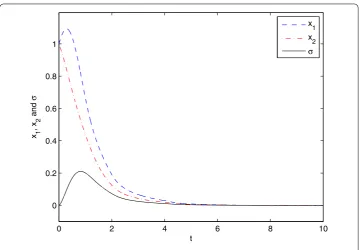
The numerical simulation is carried out by Matlab. Suppose the initial condition is [x(t)x(t)σ()]T= [ ]T,t∈[–h, ]. The state response of system () is shown in Fig-ure .
It can be seen from Figure that the zero solution of system () is asymptotically sta-ble. Changing the form off(σ(t)) and carrying out a corresponding numerical simulation demonstrate that system () is asymptotically stable as long asf(·)∈F[.,]. Thus, it is absolutely stable. This example illustrates that the simulation result is in perfect accor-dance with theoretical conclusions.
sys-Figure 1 The state response of system (6) (withf(σ(t)) = 2σ(t) + sinσ(t)).
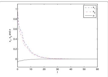
Figure 2 The state response of system (6) (withf(σ(t)) =σ2(t)).
tem () is still asymptotically stable by simulation, as shown in Figure . Therefore, it is possible to extend the absolute stability region of parameters for system (). This will be explored in our future works.
[image:15.595.118.477.352.619.2]Figure 3 The state response of the system in Example 2.
Example We still consider system (), the time delay is given by
τ(t) =
⎧ ⎪ ⎨ ⎪ ⎩
, t< , .t, ≤t≤, , t> .
The other parameters remain unchanged. Hereτ(t)≤ meansh= . Note thatτ(t) is not derivable att= andt= , but it has right and left derivative. Combined with A, we haveτ˙(t)≤.. Thus,α= .. Similarly to Example , this system is absolutely stable. By utilising Matlab, the simulation result is shown in Figure .
It is worth noting that the coefficientsA(t),B(t),b(t),c(t),ρ(t) in Example and Ex-ample are unbounded. This is the novelty of the paper. All theorems and corollaries are suitable for systems whose coefficient matrices are unbounded. Actually, for Lurie systems with bounded or constant coefficients, all results are also true. Now an example of Lurie system with constant coefficients is presented.
Example Consider the time-varying delay Lurie indirect control system with constant coefficients
⎧ ⎪ ⎪ ⎪ ⎪ ⎪ ⎪ ⎪ ⎪ ⎪ ⎪ ⎪ ⎨ ⎪ ⎪ ⎪ ⎪ ⎪ ⎪ ⎪ ⎪ ⎪ ⎪ ⎪ ⎩
˙
x(t)
˙
x(t)
=
–. .
. –
x(t)
x(t)
+
. .
. .
x(t–τ(t))
x(t–τ(t))
+
fσ(t),
˙
σ(t) =– –
x(t)
x(t)
– fσ(t),
whereτ(t) = + .sint,f(·)∈F[.,]. Here,
A(t) =
–. .
. –
, B(t) =
. .
. .
,
b(t) =
, c(t) =
– –
, ρ(t) =
are all constant matrices or constants.
Now we verify that this system satisfies all the conditions of Theorem .
First, it is obvious that ≤τ(t)≤. =h,τ˙(t) = .cost≤. < . We haveα= .. Thus, A is satisfied. Then letP=G=I, it follows that
PA(t) +AT(t)P+G=
–. .
. –
.
It is easy to obtain
λPA(t) +AT(t)P+G≤–. +√..
Thus, we have
ξ=δ(t) = . –√..
Then, A is satisfied. In addition,
PB(t)
√
δ(t)( –α)λmin(G) =
. +√.
.(. –√.)
< .,
Pb(t) +c(t)
δ(t)ρ(t) =
√
.
(. –√.) < ..
Hence, we haveη= .,γ = . in A.
It is clear that η+γ = . < , which means that the conditions of Theorem are satisfied. The conclusion could be made that system () is absolutely stable. Let
fσ(t)= σ(t) +sinσ(t).
Suppose the initial condition is [x(t)x(t)σ()]T= [ ]T,t∈[–h, ]. The simulation result is obtained using Matlab, as shown in Figure .
Figure indicates that the zero solution of system () is asymptotically stable. This veri-fies theoretical results. Changingf(σ(t)) to simulate yields that system () is asymptotically stable so long asf(·)∈F[.,],i.e., system () is absolutely stable. Thus, the results in this paper are true for Lurie systems with constant coefficients.
Figure 4 The state response of system (8).
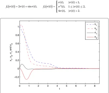
Example Consider the time-varying delay Lurie indirect control system with variable coefficients and two nonlinearities
˙
x(t) =A(t)x(t) +B(t)x(t–τ(t)) +i=bi(t)fi(σi(t)),
˙
σi(t) =cTi (t)x(t) –ρi(t)fi(σi(t)) (i= , ),
()
whereτ(t) = + .sint,fi(·)∈F[.,],i= , and
A(t) =
–t– t
–t–
, B(t) =
⎡ ⎣
t
t
⎤ ⎦,
b(t) =
√ t t
, b(t) =
–t
t
,
c(t) =
–t
, c(t) =
t
–t
,
ρ(t) =t+ , ρ(t) = t+ .
Now we verify that this system satisfies all the conditions of Corollary .
Firstly, it is obvious that ≤τ(t)≤. =h,τ˙(t) = .cost≤. < . We know thatα= .. Thus A is satisfied.
Then letP=G=I, it follows that
PA(t) +AT(t)P+G=
–t t+
t+ –t
It is easy to obtain
λPA(t) +AT(t)P+G≤–t+√t+ t+ . Further, letT= . Then, whent>T, we have
λPA(t) +AT(t)P+G< –t< –.
Thus A is satisfied withδ(t) = t,ξ= –. In addition,
lim
t→∞
PB(t)
√
δ(t)( –α)λmin(G) =lim
t→∞
√
t
√t·.=
√
,
lim
t→∞
Pb(t) +c(t)
δ(t)ρ(t) =tlim→∞
. +√t
√
t(t+ )= ,
lim
t→∞
Pb(t) +c(t)
δ(t)ρ(t) = .
We recall the fact that the upper limit always exists if the limit exists, and it is equal to the limit value. Hence, for A we haveη¯=√
,γ¯=γ¯= .
It is clear thatη¯+γ¯+γ¯=√< . Thus, all the conditions in Corollary are satisfied, that is, system () is absolutely stable.
In order to carry out the numerical simulation, let
f
σ(t)= σ(t) +sinσ(t), f
σ(t)=
⎧ ⎪ ⎨ ⎪ ⎩
σ(t), |σ(t)|< ,
[image:19.595.117.479.409.718.2]σ(t), ≤ |σ(t)| ≤, σ(t), |σ(t)|> .
Suppose the initial condition of the system is given by
x(t) x(t) σ() σ()T= T, t∈[–h, ].
With the aid of Matlab, the state response of system () is shown in Figure . It illustrates that the numerical simulation result is completely consistent with the theoretical conclu-sion.
5 Conclusion
The absolute stability problem of time-varying delay Lurie indirect control systems with variable coefficients has been investigated in this paper. Based on Lyapunov stability the-ory, some sufficient conditions and several simple and practical corollaries have been ob-tained. The results in this paper are especially applicable to checking the absolute stability of time-varying delay Lurie indirect control systems with unbounded coefficients. The validity of the proposed criteria has been demonstrated by numerical examples.
Competing interests
The authors declare that they have no competing interests.
Authors’ contributions
The authors have made the same contribution. All authors read and approved the final manuscript.
Author details
1School of Mathematics and Physics, University of Science and Technology Beijing, Beijing, 100083, China.2Leeds
Sustainability Institute, Leeds Beckett University, Leeds, LS2 9EN, UK.
Acknowledgements
This work was supported by the National Natural Science Foundation of China (grant number 61174209).
Received: 16 August 2016 Accepted: 18 January 2017
References
1. Lur’e, AI, Postnikov, VN: On the theory of stability of control system. Prikl. Mat. Meh.8(3), 283-286 (1944) 2. Liberzon, MR: Essays on the absolute stability theory. Autom. Remote Control67(10), 1610-1644 (2006)
3. Gelig, AH, Leonov, GA, Fradkov, AL: Nonlinear Systems. Frequency and Matrix Inequalities. Fizmatlit, Moscow (2008) 4. Lur’e, AI: Some Nonlinear Problems in the Theory of Automatic Control. H. M. Stationery Office, London (1957) 5. Aizerman, MA, Gantmaher, FR: Absolute Stability of Regulator Systems. Holden-Day, San Francisco (1964) 6. Xie, H: Theories and Applications of Absolute Stability. Science Press, Beijing (1986)
7. Khusainov, DY, Shatyrko, AV: Absolute stability of multi-delay regulation systems. J. Autom. Inf. Sci.27(3), 33-42 (1995) 8. Chen, W-H, Guan, Z-H, Lu, X-M: Absolute stability of Lurie indirect control systems with multiple variable delays. Acta
Math. Sin.47(6), 1063-1070 (2004)
9. Gan, Z-X, Ge, W-G: Absolute stability of a class of multiple nonlinear Lurie control systems with delay. Acta Math. Sin. 43(4), 633-638 (2000)
10. Tian, J, Zhong, S, Xiong, L: Delay-dependent absolute stability of Lurie control systems with multiple time-delays. Appl. Math. Comput.188(1), 379-384 (2007)
11. Cao, J, Zhong, S: New delay-dependent condition for absolute stability of Lurie control systems with multiple time-delays and nonlinearities. Appl. Math. Comput.194(1), 250-258 (2007)
12. Nam, PT, Pathirana, PN: Improvement on delay dependent absolute stability of Lurie control systems with multiple time delays. Appl. Math. Comput.216(3), 1024-1027 (2010)
13. Daryoush, BS, Soheila, DC: Improvement on delay dependent absolute stability of Lurie control systems with multiple time-delays and nonlinearities. World J. Model. Simul.10(1), 20-26 (2014)
14. Shatyrko, A, Diblík, J, Khusainov, D, R˚užiˇcková, M: Stabilization of Lur’e-type nonlinear control systems by Lyapunov-Krasovskii functionals. Adv. Differ. Equ.2012, 229 (2012)
15. Wang, T-C, Wang, Y-C, Hong, L-R: Absolute stability for Lurie control system with unbound time delays. J. China Univ. Min. Technol.14(1), 67-69 (2005)
16. Zeng, H-B, He, Y, Wu, M, Feng, Z-Y: New absolute stability criteria for Lurie nonlinear systems with time-varying delay. Control Decis.25(3), 346-350 (2010)
17. Liu, P-L: Delayed decomposition approach to the robust absolute stability of a Lur’e control system with time-varying delay. Appl. Math. Model.40(3), 2333-2345 (2016)
18. Shatyrko, AV, Khusainov, DY: Absolute interval stability of indirect regulating systems of neutral type. J. Autom. Inf. Sci. 42(6), 43-54 (2010)
20. Shatyrko, A, van Nooijen, RRP, Kolechkina, A, Khusainov, D: Stabilization of neutral-type indirect control systems to absolute stability state. Adv. Differ. Equ.2015, 64 (2015)
21. Liao, F-C, Li, A-G, Sun, F-B: Absolute stability of Lurie systems and Lurie large-scale systems with multiple operators and unbounded coefficients. J. Univ. Sci. Technol. B31(11), 1472-1479 (2009)
22. Wang, D, Liao, F: Absolute stability of Lurie direct control systems with time-varying coefficients and multiple nonlinearities. Appl. Math. Comput.219(9), 4465-4473 (2013)
23. Liao, F, Wang, D: Absolute stability criteria for large-scale Lurie direct control systems with time-varying coefficients. Sci. World J.2014, Article ID 631604 (2014). doi:10.1155/2014/631604
24. Burton, TA: Uniform asymptotical stability in functional differential equations. Proc. Am. Math. Soc.68(2), 195-199 (1978)
25. Burton, TA: Stability and Periodic Solutions of Ordinary and Functional Differential Equations. Academic Press, New York (1985)