Citation:
Altahhan, A (2016) Self-reflective deep reinforcement learning.
Proceedings of the
Inter-national Joint Conference on Neural Networks.
pp.
4565-4570.
ISSN 2161-4407 DOI:
https://doi.org/10.1109/IJCNN.2016.7727798
Link to Leeds Beckett Repository record:
http://eprints.leedsbeckett.ac.uk/4503/
Document Version:
Article
Creative Commons: Attribution 4.0
Electronic ISBN: 978-1-5090-0620-5 USB ISBN: 978-1-5090-0619-9 Print on Demand(PoD) ISBN:
978-1-5090-0621-2
The aim of the Leeds Beckett Repository is to provide open access to our research, as required by
funder policies and permitted by publishers and copyright law.
The Leeds Beckett repository holds a wide range of publications, each of which has been
checked for copyright and the relevant embargo period has been applied by the Research Services
team.
We operate on a standard take-down policy.
If you are the author or publisher of an output
and you would like it removed from the repository, please
contact us
and we will investigate on a
case-by-case basis.
Self-reflective Deep Reinforcement Learning
Abdulrahman Altahhan
School of Computing, Electronics and Math. Coventry University
Coventry, UK.
Abstract— In this paper we present a new concept of self-reflection learning to support a deep reinforcement learning model. The self-reflective process occurs offline between episodes to help the agent to learn to navigate towards a goal location and boost its online performance. In particular, a so far optimal experience is recalled and compared with other similar but suboptimal episodes to reemphasize worthy decisions and deemphasize unworthy ones using eligibility and learning traces. At the same time, relatively bad experience is forgotten to remove its confusing effect. We set up a layer-wise deep actor-critic architecture and apply the self-reflection process to help to train it. We show that the self-reflective model seems to work well and initial experimental result on real robot shows that the agent accomplished good success rate in reaching a goal location.
Keywords— self-reflective deep reinforcement learning; deep learning; actor-critic; neural networks; robot navigation;
I. INTRODUCTION
On-line reinforcement learning agents is difficult to train. It takes long to train because the agent does not have direct answer to the input in hand, it has to rely on own assessment of how good or bad the last action was (in the long run) to achieve a goal. For real world agent the difficulty is escalated due to partial observability and variability of experience as well as unfeasibility of deliberate repetition of this experience. Experiences vary from state and action perspectives. Subsequently, even when the agent starts form the same position and takes the same action the outcome is going to vary slightly due to the continuum of possible states at any location and due to inaccuracy of actions taken. This is especially true for agents with loos mechanics which are encountered in games and DYI robots. Moreover, it is physically difficult or undesirable to let the agent run through many episodes. Therefore, the agent needs to maximize the advantage of available experience with the least amount of time and repetition; hence offline reflection on past experience can play an important role to mitigate these difficulties.
II. THE MODEL
A. Actor-critic and Neural Networks
We consider actor-critic architecture to tackle the above problem. This architecture is interesting because it allows for explicit natural separation of concern between a performer, that tries to learn the best set of actions in certain situations, and a critic that tries to maximize overall future gain strategically. As we shall see later a specific advantage of the proposed
architecture is that it unifies both the actor and the critic in one neural network that can be readily trained using backpropagation. For the learner everything can be summed up in terms of a reward signal whether it is positive (success in reaching the goal) or negative (increased number of steps). Any negative rewards (cost) can be thought of as positive and the target would be to minimize the sum of future cost. Equally, if the agent uses only positive rewards then it would need to maximize the sum of the expected accumulated future rewards.
B. Operating under Positive and Negative Rewards
Mixing both negative and positive cost and rewards has its own perceived advantages such as enriching the agent experience, possible shortening of the training phase (instead of training through two consequent phases one for reward and one for the cost) and adding a more natural touch to the behaviour of the agent even during training. However, problems arise due to conflict of interest intrinsic in both forms. If we assign one reward function that encompasses and mingles cost and reward in each step then it would be difficult for the agent to trace what went wrong or right and what decision caused a bad or good experience in order to self-reflect on own actions.
C. The Problem Scenario
D. Self-reflective Learning
When pure cost (negative) function is considered, then early bad decisions have more effect on generating bad experience. Conventional eligibility traces help recognize this effect exactly; they put more emphasis on the early decisions so that those decisions get what they deserve of blame. Equally, when using a pure reward (positive) function, late decisions has more effect on finalizing the task and one might want to increase their effect to receive the praise they deserve to finalize the task. Conventional eligibility traces do not stress this effect except when the reward they gain is very big in comparison with other rewards of other steps. Therefore, we will apply relatively high rewards for the end of the episode. More importantly we will follow online learning approach, (that is happening during the episode) by an offline learning phase (that occur between episodes) to further emphasize the effect of good actions that lead to finalizing the task.
At the same time, when the experience is not good (agent took very long to reach the target or did not reach it in the maximum allowed number of steps) at the end of the episode the model rewinds the learning that took place by reverting the weights to their original values at the start of the episode. This is because such episodes are not fit for the agent to learn from, they will be discarded. We register the parameter changes (learning) that took place and we simply undo them and repeat the episode. We argue that the above is more like how human and animal learn from their experience. Overall we do not consider every single attempt (episode) that we do. Our brain only stimulates learning when a novel and exciting thing happen such as when the problem is solved in a shorter than usual path (relative to past experience).
So self-reflective learning occurs after each episode. If the episode is particularly good the agent reflects back to emphasize the learned lesson (either by coincidence or by some action that had a greater effect than expected). The self-excitement comes from these outcomes which stimulate remembering what has been done. We do exactly the same in our model. When a particular episode is good it provokes the agent to ponder what it has done well. So it needs either to remember the whole path and analyze it to know what has led to the success/failure as if the agent is rewinding the video of past experience and learn from it. We do this by registering the whole experience in a two conjugate gradient eligibility traces one for the actor and one for the critic, as well as by registering the exact accumulated changes done on the neural network parameter on two learning traces one for the actor and one for the critic. The four traces condense the past experience and allow us to apply the learning experience again at the end of the episode when the episode has proved to be optimal in relation to past experience. It should be noted that in the case of off-line updates and if one is using a toolbox with ready neural network structure then one can simply store the chain of vector features and estimated target value functions pairs (Fyt, VTt): VTt =rt+1 + γVt+1 where Vt+1 is the estimated value function for Fyt+1. And once these has been combined with conjugate gradient updates then it has been proven in [14] that this is indeed equivalent to a conjugate gradient eligibility traces.
Eligibility traces places more emphasis on the early actions which makes sense for online learning. For the offline case we would like to put more emphasis on the latest actions that helped the agent to reach the goal. We would like to do that before amalgamating the experience with further chain, hence online is ideal. However, for our case we want a stronger mechanism.
E. Deep Feature Represntation
Deep learning has been shown to overcome the bottleneck representation problem that has long set back the success of machine learning applications [9, 10]. This is especially important for RL since RL normally takes a long time to converge (although speeding approaches have been developed for the problem under consideration [17]). Deep learning showed very good results when combined with supervised learning [11, 12]. When combined with RL it is also believed to have a good potential [18, 19].
Our model starts by learning a concise and reduced feature representation. The model obtains a reduced representation in the first episode by deep convolutional neural network that is translation invariant as in [13, 21]. First, a set of random patches are extracted from the set of images collected in the explorative episode, then a set of weights are trained using those patches as an input and output for an autoencoder in order to extract the most resilient and important features in the environment (those images are representative for the environment since the agent is let to run around in this explorative episode to cover as much of the environment as practical). Then a set of filters are built using the strapped weights of the first autoencoder layer. The number of filters = patch_pixles2 × 3 (patch_size × channels). Each image received by the agent then will be convoluted by the filters of the autoencoder to build a set of features maps, which are then pooled (features neighborhood averaged) to reach the final set of features. The model is then shrinks the whole architecture to fit the new reduced number of features, and this concludes the deep learning phase for the feature representation layer. The explorative episode aligns with how animals normally explore a place by looking around.
F. Deep Reinforcemnet Learning Model
As it has been mentioned, the model adopts a special type of Combined Deep-Actor-Critic architecture that seamlessly unifies and integrates the policy learning process which is suitable for deep action learning [16]. In each step, after the actor layer takes its input form the deep convoluted and pooled layer, it then decides to do a certain action, accordingly the critic layer punishes or rewards the actor depending on the reward it receives form the environment.
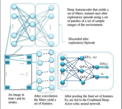
Formally, the presented model uses the following components/stages shown in Fig. 1:
Goal representation: We said earlier that that the brain hard wires the scenes to itself and compare it with the look of the home. To do so we need to run into an initial identification stage that identifies the home and embeds its views in the agents’ goal-identification behaviour. To do so the agent takes n snapshot for the home in different orientation and distances. The feature vector is calculated in two stages; preliminary and primary:
[image:4.595.31.292.286.519.2]In the preliminary stage the agent learns a set of useful filters using the method mentioned in previous section. The deduced filters will be convoluted over each coming image in each time step. The filters are calculated at the end of the first explorative episode. This stage can be extended to span more than one episode to give a denser environment sampling. Then the model shrinks the whole architecture to fit the new reduced number of features. This concludes the deep learning stage for the feature representation layer. This stage is done once and will not be repeated.
Fig. 1. The Blended Deep-Actor-Critic Neural Network Components and Model’s Stages.
Each image was normalized and the number of patches were chosen to be 1000 and were selected randomly form the exploratory episode environment dataset. The size of the patch was chosen to be 6 hence input size for the auto-encoder is 6×6×3 (RGB channels) =108. The number of filters (i.e. number of neurons in the hidden layer) were chosen be 9. The convolution procedure was set to go iteratively as a 2D patch_size2 matrix that has all the weights for a specific neuron (related to a specific channel).
The dimension of the features
f is d1×d2×f where d1 andd2 are the dimensions of the stride and f= is the number of filters. The dimension of the reduced features
f is n. Thefeatures
fare then used to calculate a similarity indexdeep-NRB:
is a deep representation of the stored image j
with filter f. is a channel c view of stored image j, and
is deep representation of channel c of current image
st, while σ is a variance. The similarity measure that specifies
the termination of the episode and is given by to be normalized radial basis function DeepNRB s n
s nf f t
t)
1(
. Thismeasure has been used along with two thresholds to set the stopping and approaching conditions for the agent. Using deep DeepNRB The reward function is given as a combination of step cost in addition to a reward for going towards (approaching) the goal as well as a reward for reaching the goal [14].
Two important aspects related to the actions: when the agent turns, it will acquire higher costs than when it goes straight. This has the desired consequence of suppressing unnecessary turns and emphasizing going straight. Also a punishment for taking any action that leads to a reactive behavior has been set. This reduces the costal behavior and encourages going directly towards the goal.
G. Deep Blended Actor-critic Layered Architecture
The input feature layer is followed by an actor layer. The actor outputs three distinctive estimations of action-value function; each stands for one action. The three output of the actions-value function are followed by a value function layer that calculates the value function for the policy of the actor. This last layer represents the critic. At the same time the three action-values are passed through a winner takes all function were the max value will be taken as the winner action at as shown in Fig. 1. The learning occurs on the form of a reward signal that is fed first to the value function then back propagated to the previous actor layer. Fig. 1 shows the layers, stages and component of the system.
By constructing the actor-critic architecture as two consequent layers and by allowing the second layer to act as a critic that contemplates the consequences of the actions of the actor layer and sends a conjugate gradient signal to it to indicate how well its current policy is, we created a deep blended actor-critic architecture in one sound system that depends on two eligibility traces. The value function layer itself is taking its feedback form the reward function. The action layer can learn independently of the critic layer by utilizing an action-value function approach (for example learning can occur on the wining action only). Whereas, the critic layer cannot process independently since it needs the actor layer to calculate the value function. However, the critic layer can be trained independently by not back propagating to the actor layer. In that sense the learning process can be thought of as a layer by layer learning or deep learning enabled. In the future we will explore training each layer independently by freezing learning in each layer and then fine-tune by utilizing the presented approach. So this model is deep
2
2
ˆ 2
) , ( ) ( exp
) , (
s c j hf st c hf vc j
t f
v
(
c
,
j
)
h
f) , (c j v
s
(
c
)
h
i tAn image at time t and its strides.
Fyt
for …
…
… …
…
…
…
…
…
…
…
…
…
After convolution the filters yield a set of features.
After pooling the final set of features Fyt are fed to the Combined
Deep-Actor-critic neural network V Q(Fyt , al)
Q(Fyt , ar)
Q(Fyt , af)
Q(Fyt , ar) at V(Fyt)
Deep Autoencoder that yields a set of filters, trained once after exploratory episode using a set of patches of a set of sample images of the environment.
Discarded after exploratory Episode
…
in terms of its feature representation and has the potential to be deep in terms of its action representation.
H. Actor-critic Combined Network with Double Eligibility Traces
In this section we show the derivation of the learning formulae for the layered actor-critic architecture. When function approximation techniques are used to learn a parametric estimate of the value function V(s), ( )
t t s
V is expressed in terms of a set of parameterst. The mean
squared error performance function [4] can be used to drive the learning process:
S s t tt MSE pr s V s V s
Error ( ) ( ) ( ) ( )2
) (s
pr is a probability distribution weighting the errors
22 ) ( ) ( )
(s V s V s
Errt t
of each state s, and expresses
the fact that better estimates should be obtained for more frequent states. The function
t
Error needs to be minimized in order to find an optimal solution *
t
that best approximates the value function. For on-policy learning if the sample trajectories are being drawn according to pr through real or simulated experience, then one can concentrate on minimizing the error function Err2(s)
t . By using two layered neural
network (one hidden layer and an output layer) and two sigmoid activations the reinforcement learning problem of learning an approximation of the value function and the action-value function can be written as:
I i t
t iw i
Q t t e s V 1 ) ( ) ( 1 1 ) ( K k t
t k ik
F t e i Q 1 ) , ( ) ( 1 1 ) (
The update rule can be written as
t t t d 2 1
, dt is a vector that drives the search for *
t
in the direction that minimizes the error functionErrt2(s), and 0t 1 is a step
size. This direction can be chosen in several ways. For example, the update rules for weights that go opposite to the gradient direction are:
) ( ) ( ) ( ) ( ) ( i w s V s V s V i w t t t t t t t t
) , ( ) ( ) ( ) ( ) , ( k i s V s V s V k i t t t t t t tt
By bootstrapping and using the rt1Vt(st1)as an approximation for V(st) and be defining
) ( ) ( 1
1 t t t t
t
tr V s V s
we have
) ( ) ( ) ( i w s V i w t t t t t t
) , ( ) ( ) , ( k i s V k i t t t t tt
It should be noted that these rules are approximate gradient descend.
I. Conjugate Gradient Updates
In this section we extend the actor-critic setting to allow for two conjugate gradient eligibility traces. We will follow the same analogy of [14 and 16]. We update the error in (6) opposite to the direction of the conjugate gradient of the output and the action layers hence:
) ( ) ( ) ( )
( p1i
i w s V Err i
w t t
t t t t t
t
(, ) ) , ( ) ( ) ,
( p 1ik
k i s V Err k
i t t
t t t t t
t
Where β and β` factor can be specified in several ways, for example for β we have:
1 1 1 ) ( t T t t T t HS t p g g g 1 1 ) ( t T t t T t FR t g g g g 1 1 1 ) ( t T t t T t PR t g g g g Conjugate gradient direction for the critic
pt gwt tpt1
t wErr
p
0
) ( ) ( ) ( ) ( 2 ) ( 2 ) ( k s V s V s V s Err g t t t t t t t t k t t
t t t t t t t t w w w s V s V s V s Err g t t 2( ) 2 ( ) ( ) ( ) Similar set of formulae can be defined for the actor.
Now we define ( ) 1
conj t
e and ( ) 1
conj t
e as follows:
1 )
(
1
t
t t conj t t t p Err e
1
) ( 1 t t t conj t t t p Err
e
We can evaluate this in several ways; for example:
t t t t Err t t t t Err
The updates can be rewritten as:
( ) ) ( ) ( conj t t t t tt V s V s e
w
) ( ) ( ) ( )(k V s V s e(conj) k
t t t t t
t
) (
1 )
( ( ) conj
t t t t t t conj t e w s V
e
( ) ) ( ) ( ) ( ( ) 1 k e k s V k e conj t t t t t t
t
The above shows that eligibility traces are in fact independent of the error that we use whether it is approximation or exact. In fact, it distinctively shows that for any error there is an eligibility trace that coincides with the conjugate gradient; it varies with the reverse of the error.
t t
,
can be chosen in several ways other than the presented. In general (PR)t
has been shown to perform better due to its stability for nonlinear error functions [20].
varies with the error no matter what type of error we are using, and that the reward discount should be varied according to the direction of the conjugate.
For example, if we approximate the error using two layers with bootstrapping and using the rt1Vt(st1)as an
approximation for V(st)we have:
( )
1
conj t t t
t e
w
t(k) t t et1(k)
( )
1 )
( ( ) conj
t t t t
t t conj
t e
w s V
e
) ( )
( ) ( )
( e 1 k
k s V k
e t
t t t
t
Were δ being the temporal difference error. Eligibility traces in reinforcement learning framework is similar to the momentum for supervised learning. It establishes a way to accommodate previous updates into current updates to guide the search for the local optima. In RL it traces blame of current decision back to older decisions that lead to the current situation. Finally, a regularizer
has been multiplied by the two parameter sets to discount the old values of the parameters (hence prevent overfitting).When an episode has been signaled as an optimal (based on its number of steps being minimal), the learned experience was emphasized after the episode has finished in an offline learning fashion as follows:
ep ep
T
t t T
ep w w
w
1
ep
ep
T
t t T
ep k k k
1 ) ( )
( )
(
Also when an episode has been signaled as bad (its number of steps is worst), the model rewinds the learning done through this experience: This was allowed after j initial non-reversing episodes.
/ ) (
1
ep ep
ep
T
t t T
T w w
w ( ) ( ( ) ( ))/ 1
ep
ep ep
T
t t T
T k k k
III. EXPERIMENTAL RESULTS
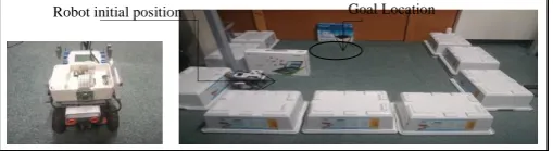
[image:6.595.305.563.577.673.2]Fig. 2 shows the used robot and its environment. It is basically an updated version of Lego Mindstorms that has been used with additional camera module and processing unit that was mounted and attached on top of it. This robot has a relatively low level of sophistication in terms of the motor commands, balance, senor reading as well as its shape. RWTH- Mindstorms NXT Toolbox has been used to provide the sensory reading and the actuator commands for the NXT robot.
Fig. 2. Left: A snapshot of the built robot with its sensors, actuators, and camera module. Right: The training environment.
The robot was let to train for 30 episodes and to cool down for 5 episodes. Each episode starts by going from behind the barrier location in the environment to the goal/home location. It was allowed to run for a 500 steps before the episode is considered a failure. Images with resolution of 160×120 were sent form a Raspberry PI module wirelessly to an off-board computer for processing. Learning took place in the off-board computer then the action decision is sent to the actuators of the robot via its Bluetooth. Threshold that specifies reaching the goal was set to 0.97%.
A. Agent Learning Behavior and Convergence
Fig. 3 shows the number of steps in each episode. Three distinguished stages can be identified; each marks a certain behavioral learning. Each stage is distinguished through its average number of steps (red bar). Although the number of steps needed to reach the goal is inevitably varying, however each stage can be recognized by a different average. In the first 9 episodes the agent did not apply any self-reflection and the average number of steps (recognized by the red doted bar) were the highest (51.5). The second stage started from episode 10 onwards where agent did apply self-reflection on episodes 10, 14, 30 (recognized by green). Those were relatively minimal comparing to past experience, the condition was set to apply self-reflection if the finished episode has steps ≤ second minimal past episode. The average in this stage is 25.05 steps. The third stage is form 31 onwards where the agent just enjoyed following its learned policy with no online learning, average was 13.4 steps only. Agent applied self-reflection on episode 31. Episode 22 was suitable for rewinding but it was not applied due to a high number of steps in the first stage. This proposes a future change of comparing only within the self-reflection window rather than all previous episodes.
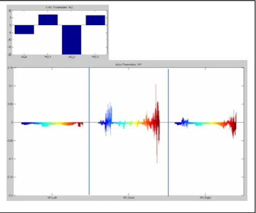
[image:6.595.37.292.620.689.2]An important thing to realize is that after the agent learns a suitable policy in the first 30 episodes, its performance stabilizes on an optimal policy with minimum number of steps the agent needed to reach the goal. This is a distinguished trait of this model. Bearing in mind that no experience can be reproduced by the agent, even when the agent finalizes the learning stage, a developmental behaviour can be realized. First, the agent developed a primitive behavior of moving forward and occasionally turning to minimize its cost. Then the agent started to develop inclination of going forwards and turn with some costal behaviour. In fact, turning in one direction was preferred and enforced over the other actions. This is particularly evident when we look at the overall size of the actor parameters in Fig 4.
Fig. 3. The convergence to a stable number of steps is shown to develop; the red bar shows the avergae number of steps needed for each stage to reach the goal.
Initial learning
Self-reflection window
Fo
llo
w
Po
licy
The number of episodes is envisaged (as was evident in the simulation in [14, 15 and 16]) to show a pattern of convergence towards minimal number of steps if the robot where left to run for a very long time. This was not needed in this realistic robotics scenario since the agent reached a good policy in 30 episodes only. However, due to time and physical constraints, this was difficult to do and a powerful and fast model was developed to reach a suitable strategy. The experiments were conducted by starting always form roughly the same position. The variation is due to the different learning stages as well as due to the continuum of possible states at any location and due to inherited inaccuracy of actions taken (due to the mechanics of the used robot). Our results show that out of 35(30 training + 5 testing) times, the agent reached the goal location in all of them but 7 with not a desired orientation; the goal was not directly inside the visual field of the robot. Hence, it can be concluded that the success rate is 35/35 ≈ 100% while goal orientation recognition is 80%.
Fig. 4. The model learned parameters for the actor and the critic; three actions is shown where gradient eligibility trace is used; a tendency towards going forward then turning left is developed by the agent.
B. Summary and future work
In this paper an initial self-reflective learning model that depends of deep combined actor-critic layered architecture has been introduced. Self-reflection entails that the agent should further ponder on negative and positive experience and should take advantage of negative and positive costs and rewards by either duplicating the learning process for successful experience or forgetting it for bad ones. Relatively optimal past experience is recalled, offline between episodes, and compared with other similar but suboptimal episodes to single out which decision was particularly good and positively be reemphasized, hence suboptimal decision is singled out and deemphasized. Equally, relatively bad experience is forgotten, offline between episodes, to remove its confusing effect. In the future we will be looking at different ways to formalize the approach further and conduct more experiments to verify its suitability for different scenarios. Also it is intended to show some other interesting properties of the model such as
convergence and the relationship between deep feature learning and deep action learning.
REFERENCES
[1] A. Vardy and R. Moller, “Biologically plausible visual homing methods based on optical flow techniques”, Connection Science, vol. 17, pp. 47– 89, 2005.
[2] N. Tomatis et al, “Combining Topological and Metric: a Natural Integration for Simultaneous Localization and Map Building”, presented at Proc. Of the Fourth European Workshop on Advanced Mobile Robots (Eurobot), 2001.
[3] Jochen Zeil, “Visual homing: an insect perspective, Current Opinion in Neurobiology”, Volume 22, Issue 2, pp. 285-293, ISSN 0959-4388, April 2012
[4] R. S. Sutton and A. Barto, “Reinforcement Learning, an introduction”, Cambridge, Massachusetts: MIT Press, 1998.
[5] V. Konda and J. Tsitsiklis, “Actor-Critic algorithms”, presented at NIPS 12, 2000.
[6] O. Ziv and N. Shimkin, “Multigrid Methods for Policy Evaluation and Reinforcement Learning”, presented at IEEE International Symposium on Intelligent Control, Limassol, 2005.
[7] C. Zhang at al, “Efficient multi-agent reinforcement learning through automated supervision”, presented at International Conference on Autonomous Agents Estoril, Portugal, 2008.
[8] S. Bhatnagar et al, “Incremental Natural Actor-Critic Algorithms”, presented at Neural Information Processing Systems (NIPS19), 2007. [9] G. Hinton et al, “A fast learning algorithm for deep belief nets”. Neural
Computation,18(7):1527–1554, 2006.
[10] A. Coates et al, “An Analysis of Single-Layer Networks in Unsupervised Feature Learning”, in AISTATS 14, 2011.
[11] P. Vincent et al, “Extracting and composing robust features with denoising autoencoders”. In ICML, 2008
[12] A. Ng et al (2010), Tutorial in Deep Learning: Stanford University [Online]. Available: http://ufldl.stanford.edu/tutorial/
[13] Y. LeCun et al, “Learning methods for generic object recognition with invariance to pose and lighting”. In CVPR, 2004.
[14] A. Altahhan, “A Robot Visual Homing Model that Traverses Conjugate Gradient TD to a Variable λ TD and Uses Radial Basis Features”, in Advances in Reinforcement Learning, A. Mellouk, Ed. Vienna: InTech Education and Publishing, 2011, pp. 225-254.
[15] A. Altahhan, “Robot Visual Homing using Conjugate Gradient Temporal Difference Learning, Radial Basis Features and A Whole Image Measure”, International Joint Conference on Neural Networks (IJCNN), Barcelona, Spain, ISBN: 978-1-4244-6916-1, 2010.
[16] A. Altahhan et al, “Deep Feature-Action Processing with Mixture of Updates”, Neural Information Processing Volume 9492 of the series Lecture Notes in Computer Science pp 1-10, 2015
[17] A. Altahhan, A Fast Learning Home Aware Robot Navigation Learning Using Simple Features and Variable Lambda TD, 2014 International Joint Conference of Neural Network (IJCNN), China, IEEE, pp ISBN:10.1109/ IJCNN.2014.6889845, 2014.
[18] A. Altahhan, ‘Navigating a Robot through Big Visual Sensory Data’, INNS Conference on Big Data 2015 Program San Francisco, CA, USA 8-10 August, Procedia Computer Science, Volume 53, Pages 478–485 2015.
[19] V. Mnih et al, Playing Atari with Deep Reinforcement Learning, NIPS Deep Learning Workshop 2013.
[20] Nocedal, Jorge, Wright, Stephen, 2006, Numerical Optimization, Springer-Verlag New York, 978-0-387-30303-1, 2nd Edition
[21] R. S. Sutton et al, A new Q(lambda) with interim forward view and Monte Carlo equivalence, Proceedings of the 31 st International Conference on Machine Learning, Beijing, China, 2014. JMLR: W&CP volume 32, 2014