MYOPIC SELECTION*
P. A. Geroski
London Business School, UK
M. Mazzucato The Open University, UK
Abstract:
The severity of selection mechanisms and the myopia of selection are explored through a duopoly model where one firm tries to move down a learning curve in which costs are initially higher than its rival’s but ultimately much lower. A trade-off is found between catch-up time and asymptotic market share: the more severe are selection pressures, the less likely is it that the learning technology will survive, however if it does survive, the learning
technology will in the limit be more competitive the more severe are selection pressures. We explore the dynamics of the model under unit cost and strategic pricing and find that the optimal pricing rule depends on the parameters governing firm learning and market selection.
Key Words: learning by doing, selection, strategic pricing, capital markets.
JEL Classification: L1 (market structure, firm strategy and market performance), D4 (market structure and pricing).
*We are obliged to the ESRC and to an EC Marie Curie Training and Mobility of Researchers Grant (contract no. ERBFMBICT972263) for financial support, and to Luis Cabral, the editors,and the referees for helpful comments on an earlier draft.
Correspondence: Mariana Mazzucato, Economics Department, The Open University, Walton Hall, Milton Keynes, MK7 6AA, United Kingdom. Tel. 00-44-1908-654437,Email
I.
INTRODUCTION
The analogy between natural and market selection that underlies popular (and some
scholarly) notions of “competition” has inclined many to believe that an increase in the
severity of selection pressures will inhibit the willingness of firms to invest and innovate in
new technologies. The problem arises because selection based on current fitness is myopic,
and, in a market context, this means that only current performance matters. In these
circumstances, anything that increases selection pressures will concentrate attention on
current fitness, discouraging behaviour that sacrifices current performance for enhanced
future performance. In a market context, this means that increasing selection pressures will
diminish incentives to invest (e.g. in technological change).
Actually, things are not quite this simple. There are two levels of selection through
which a firm must pass if it is to survive: product market selection and capital market
selection. Product market selection operates through the mechanism of consumer choice.
Firms whose products are of good value attract customers, earn profits and use them to
expand. Although some customers take a long-sighted view and support innovative firms with
temporarily high prices, this is definitely not the general rule (particularly in consumer
markets). Capital market selection is, in principle, different. Banks and other financial
institutions will often make loans to firms who seek to improve their future competitiveness at
the risk of weakening their current financial position, and they will also loan to firms whose
current activities are unprofitable if they believe that improvements will be made in the near
future. In this sense, capital market selection may midigate some of the effects of product
market selection, making current fitness much less important in determining an enterprise’s
future growth and development than would be the case if product market selection were the
In this paper, we explore the relationship between the severity of selection
mechanisms and the myopia of selection processes using a simple simulation model of a
duopoly in which one firm tries to move down a learning curve in which costs are initially
higher than its rival’s but ultimately much lower. The intensity of product market selection is
studied by varying a parameter which denotes the degree of consumer price sensitivity: the
more price sensitive are consumers the more severe is selection. In the absence of capital
market selection, increases in market selection pressures have two opposing effects on the
decision to invest in the learning technology. On the one hand, the more severe are selection
pressures, the less likely is it that the learning technology will survive due to its higher initial
costs (and prices). On the other hand, if it does survive, the learning technology will be more
competitive the more severe are selection pressures. This second effect means that a
long-sighted lender may be willing to support such investments, particularly when product market
selection pressures are particularly strong. As a consequence, the addition of capital market
selection completely confounds the common presumption: as product market selection
pressures become more severe, the ability of the learning firm to borrow against future
performance increases and this facilitates the introduction of the learning technology. That is,
increases in the severity of product market competition increase the likelihood that the new
technology will be introduced when capital market agents are prepared to lend against future
performance.
The structure of the paper is as follows. In Section II, we introduce the model. The
main modelling challenges are the need to parameterize the severity of product market
selection pressures in a manner which makes comparative static exercises fairly transparent,
market selection. Our basic results are summarized in the form of four propositions, and these
are discussed in Section III, and Section IV contains a few concluding observations.
II.
THE MODEL
We suppose that there are two firms, i = 1,2, that there exist exogenous entry barriers
which mean that there will always only be two firms, and that the two firms price
non-cooperatively and do not collude. Firm 1 operates with a “traditional technology” which
enables it to produce output x1(t) at constant unit costs c1. Firm 2 invests in a “learning
technology” in which unit costs are initially c0 > c1, but fall with cumulative output, Q ≡Στ {x2(τ) + 1}:
c2(t) = c0Q(t)λ. (1)
λ is the learning index and is equal to logβ/log2 where β is the rate of learning and
1-β is the progress ratio.1. If we want to set our learning index close to the empirically
relevant progress ratio of .20 then we must set λ close to log.80/log2 = -.32. In the
simulation exercise below we perform comparative static exercizes using values of λ
close to .3.
Since, in principle, firm 2 could have opted to use the traditional technology, the
difference between the two firms’ initial costs, Δ≡{c0 – c1}, can be thought of as the per
period fixed (licensing) cost that firm 2 has to pay to get access to the learning technology. In
the model we use the parameter δ to denote the percentage difference in initial costs between
slow and set up costs are high (i.e. if λ is small and δ is large), then the learning technology is
unlikely to displace the traditional technology. Finally, we define t* as the time when the two
technologies achieve parity; i.e. t* satisfies c1 = c2(t*). This “switch-over point” identifies the
earliest time at which the learning technology can survive the most severe product market
selection pressures.
Since we have assumed the existence of exogenous entry barriers, selection in product
markets operates only through price competition between the two established players. Hence,
the severity of selection depends on how sensitive consumers are to price differences between
firms. There are several ways to model this. One is to suppose that all consumers are the
same, and to allow parametric variations in their elasticity of demand (or some such
parameter) to reflect variations in the intensity of selection. Another is to suppose that there
are different types of consumers, some more price sensitive than others. In this case, the
intensity of market selection pressures will reflect differences in the population mix. We have
opted for this second course. We suppose that there are a fixed number, N, consumers, and
that θ% of them are sensitive to prices (i.e. they always buy from the low priced firm). The
remaining (1 - θ)N “noisy consumers” choose randomly between the two firms regardless of
the sign or size of the price difference between them. If both firms change the same price, the
“price sensitive consumers” choose randomly between them.
This specification of demand produces a ‘kink’ in the demand facing the two firms. In
particular, if:
p1 > p2, x1 = (1 - θ)N/2 and x2 = θN + (1 - θ)N/2; (2)
p1 < p2, x1 = θN + (1 - θ)N/2 and x2 = (1 - θ)N/2.
Clearly, when θ = 1, only price sensitive consumers are present in the market, and selection
pressures are as severe as they can be. When θ = 0, on the other hand, consumers are all noisy
and they choose randomly between the two firms. In this case, no effective selection occurs.
We assume that firms do not know the value of θ and cannot identify “price sensitive”
or “noisy” consumers or discriminate between them. If this market were monopolized
recognized and θ were known to be small (i.e. when most consumers are noisy), the
monopolist will be tempted to set P→∞, driving price sensitive consumers out of the market
and taking full advantage of the rest. To rule this out, we would have to suppose that (2) is an
approximation to true demand behaviour which is accurate only in the neighbourhood of c1.
Alternatively, we could suppose that there is a large queue of potential entrants who will enter
if price exceeds some limit, p1 > c1. The duopolists in our model set prices non-cooperatively,
so there will be a strong tendency for prices to fall to the level of costs. Still if the duopolists
know that θ is small, they might price above costs. To keep the analysis tractable, we rule
this out.
It is worth making four observations on our specification of consumer price
sensitivity. First, market demand has no elasticity in this model, but the demand facing
individual firms is elastic (at least in the neighbourhood of the point at which their prices are
equal). Aside from basic tractability, this specification has the virtue of concentrating
attention on competitive pressures. Market growth is something which benefits all firms and it
also facilitates the introduction of new technologies (whose fixed costs can be spread over a
exogenously or endogenously generated market growth helps to make market selection more
difficult than it might otherwise be, and it is easy to see how the results will be affected by a
generalization along these lines.
Second, although consumers base their choice solely on price (product quality is not
introduced in the model), there are different ways that the ‘noise’ embodied in θ can be
interpreted. For example, θ can be interpreted as reflecting the degree of brand loyalty in the
market in a way that is similar to the ‘preference parameter’ used in Cabral and Riordan
(1994). In a model of a price-setting, differentiated duopoly selling to a sequence of
heterogeneous buyers with uncertain demands, they define the preference parameter as the
variance of the distribution of consumer preferences for a particular firm’s product.
Consumers buy from that firm only if the degree to which they like its product is larger than
the degree to which its price is larger than the other firm’s price. They find that the higher is
the variance of the distribution, the larger is this firm’s asymptotic market share. This is
similar to our result (below) that the lower is the degree of consumer price sensitivity, θ (i.e.
the more random is selection), the higher is the asymptotic market share of the learning firm.
The third observation relates (2) to the literature on evolutionary dynamics2. These
models often represent the selection mechanism by using a “replicator” function which
relates fitness (e.g. the difference between a firms costs and those of its rivals) to reproductive
success (e.g. changes in the firm’s market share). Since prices are related to costs (see below)
and N is fixed, it is clear that (2) is just a very specific type of replicator function linking cost
differences to market shares. Its virtue in our eyes is that it displays the mechanics of how
selection rewards fitness in a way which can be related to basic features of consumer
Finally, although we look at θ in a comparative statics framework, there are several
ways θ can be made to evolve endogenously. The degree of consumer price sensitivity could,
for example, depend on the degree to which prices differ between the two firms: when price
differences are small consumers are less price sensitive. Or it could also depend on more local
consumer behavior such as that described in Cowan et al. (1997) where consumers are
influenced by the consumption behavior of others. This can take the form of buying what the
‘best’ people bought (a group to which the individual aspires to be similar) not buying what
the ‘worst’ people bought (a group from which the individual seeks to differentiate
him/herself), or copying the buying behavior of their closest peers (Cowan et al. 1997). We
choose to keep θ exogenous for the use of clarity in the comparative statics and also because
our experiments with an endogenous θ do not significantly alter the results found. We discuss
this further below.
Capital market selection pressures describe the ability of firms to finance current costs
incurred to generate future profits. The effects of capital market selection are reflected in the
amount of money that firms can borrow, and on what terms. Our interest here is in trying to
parameterize the constraints imposed by the capital market in as simple a manner as possible.
Suppose that firm 2 incurs losses to travel down its learning curve as fast as possible. Once it
has reached unit cost parity with firm 1 (which occurs at t* and is endogenous to the model),
it can begin to earn profits to pay these losses back. If t0is the time at which these (total)
losses are offset by subsequent profits, then T≡ t0 - t* > 0 is the pay-back period. If the capital
market refuses loans with a pay-back period longer than ϕ, then increases in ϕ correspond to a
weakening in capital market selection pressures. In the limit as ϕ→ 0, we revert to a situation
ϕ is a simple measure of the extent to which capital markets alleviate (myopic) product
market selection pressures.
The final aspect of model specification is pricing. In the absence of a capital market,
firms cannot make losses and survive, and, when firms choose prices non-cooperatively, this
means that prices will be driven down to costs. In a “no-losspricing regime”, prices will,
therefore, be given by:
p1 = c1 and p2(t) = c2(t-1). (3)
where we have introduced a lag to simplify our computations. If firms can borrow on the
capital market, then firm 2 can price more aggressively, setting current losses against the
future profits which will appear when it has become more efficient than firm 1.3 For firm 2,
this means undercutting firm 1 in order to build up experience (through cumulative sales). The
very specific nature of (2) makes this “strategic pricing regime” very simple to describe.4 In
particular, what matters from the point of view of attracting consumers is that p2 is less than
p1. Since θ is exogenous, the absolute size of this difference has no effect on the demand for
firm 2’s product, and this means that all it needs to do is to slightly undercut firm 1 both
before and after t*. Hence, in this regime, prices will be given by:
p1 = c1 and p2 = c1 - ξ, for some ξ > 0.5 (4)
By way of summary, then, the model determines values of three variables of interest:
t*, the switch point at which the new learning technology becomes cost competitive with the
technology; and T≡ t0 - t* , the pay-back period when firms are allowed to price strategically.
The exogenous parameters of the model are: θ, the degree of product market selection
pressure; N, the market size; λ, the learning rate (or index); δ, the licensing cost of the
learning technology (described by the percentage difference in initial costs); ξ, the price
discount used in the strategic pricing regime; and the pricing rule used (no-loss or strategic).
In the simulations we experiment with different values of these parameters except in the case
of ξ (arbitrarily set at .005) due to the fact that the structure of (1) makes the exact value of
this parameter irrelevant.
III. THE
RESULTS
Using simulation techniques we explore the types of market structures which emerge
under different parameter conditions, where by market structure we mean the values of s* and
t*. For each set of initial conditions, we first solve for output via (2) (based on the initial
prices in [3] and [4], then for the costs (and prices) of the learning firm via (1), and then
again for output via (2) etc. In the case of strategic pricing, we also calculate the time period
t0 at which the learning firm is able to fully pay back its debt accrued by pricing above cost.
Our results can be summarized in the form of four propositions. We start by
examining the ‘no-loss’ pricing regime where firms are forced to price in a way which enables
them to break even period by period.
Proposition #1: Long run market shares, s*, and the time at which the new technology becomes established, t*, increase in θ.
The first part of this proposition follows directly from (2) without the need for any
is somewhere between 50% and 100%. If θ = 1, all consumers are price sensitive and, since
firm 2 is the high priced firm initially, it never attracts any customers. However, once θ falls
slightly below unity (i.e. some noisy consumers are present), firm 2 will attract some
customers. This, of course, happens every period, and since nothing in the model limits the
ability of firm 2 to go down the learning curve (as long as θ<1), all of this means that firm 2
will eventually become cost competitive with firm 1. The smaller is θ, the more sales it enjoys
period by period (and, therefore, cumulatively at any time t) and, when θ = 0, it captures 50%
of the market initially and in every period up until t*. In the long run when c2 < c1, and, as a
consequence, p2 < p1, the market share of firm 2 is s* = (1 + θ)/2.6 Columns 1 and 2 in Table
1 illustrate this result.
The fact that t* increases with θ is intuitively obvious as well. When θ is just slightly
below unity, firm 2 attracts only a few noisy customers per period, and, regardless of the
learning rate, this means that it will take a long time for it to accumulate enough experience,
Q, to get far enough down the learning curve to achieve cost parity with firm 1. However, the
lower is θ, the more noisy customers there are, and, consequently, the more sales firm 2 will
enjoy. All of this means that it will learn much faster than would otherwise have been the case
had θ been larger. The net effect is that t* is brought forward; i.e. as θ decreases, t* falls. This
holds for any parameter values as long as the learning firm prices at unit costs (the case of
strategic pricing is reviewed later). Columns 3-6 in Table I show this result with different
market sizes and initial cost differences and columns 3-5 in Table II with different learning
indices: in each case as θ increases, t* falls. When θ = 1, firm 2 never emerges.
The substance of Proposition #1 is that increases in selection pressure slow the arrival
of the new technology, making it harder for it to become established. This, of course, appears
to be an instance of myopic selection, and it appears to work to the disadvantage of
consumers. However, if and when the new technology becomes established, then increases in
selection pressure bring larger gains to firm 2, since stronger selection gives an increasingly
large reward to the cost efficiencies which have accompanied the introduction of the new
technology. This too reflects the workings of myopic selection, since, once again, selection is
merely rewarding superior current performance. In this case, however, myopic selection
appears to work in consumers’ interests. The bottom line, then, is that the common
presumption is (roughly) right: product market selection is myopic in the sense that it
discourages the emergence of new, superior technologies. However, myopic selection based
only on current performance differences at least has the virtue of rewarding firms who have
somehow managed to establish superior technologies on the market.
Proposition #2: The time it takes the learning technology to become established, t*, increases in its licensing costs, δ, market size, N, and decreases in the learning index, λ.
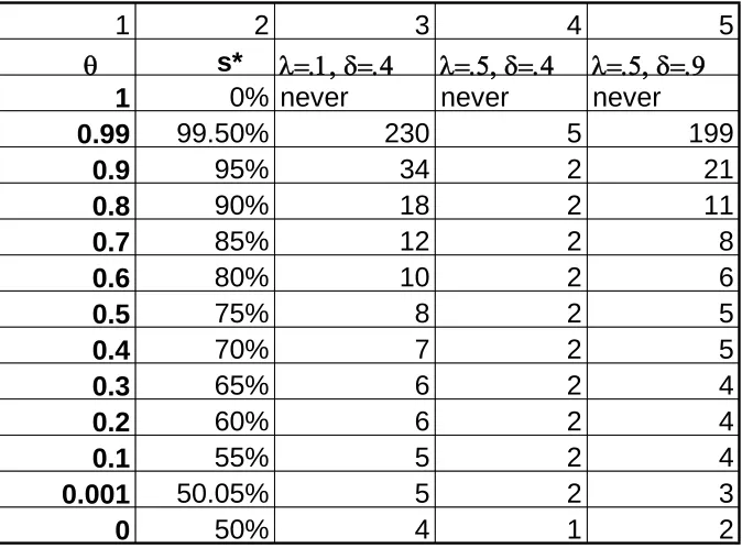
Columns 3-6 in Table I and columns 3-5 in Table II contain a range of simulations
which document the assertions in Proposition #2. Table I indicates that with a given θ, an
increase in market size (N=50⇒100) and a decrease in the initial cost difference (from δ=.5 to
δ=.4) allow firm 2 to proceed more quickly down the learning curve, causing t* to fall. Table
II indicates that this also occurs through an increase in the learning index (from λ = -.1 to λ =
-.5). Column 4 in Table II indicates that when the rate of learning is relatively high (λ=.5) it
almost doesn’t matter what the value of θ is since cost convergence occurs very quickly.
Column 5 indicates that this is less true when the initial cost difference is very large (from
follows: if the learning firm wants to obtain a fast rate of learning (to reach t* more quickly) it
will have to make a large initial investment reflected in a high δ.
TABLE II
Intuitively, these propositions are fairly easy to grasp. Licensing costs are just another
way of referring to the initial investment which firm 2 must make in the learning technology:
δ is the initial unit cost disadvantage which it accepts in order to have access to the lower
costs in the future available through learning. The higher is this initial cost penalty, the longer
it takes (ceteris paribus) to establish cost parity. Market size matters to firm 2 because the
number of consumers it serves when its price is higher than that of firm 1 is (1 - θ)N. Clearly,
the larger is the market, the more (noisy) consumers it attracts period by period for a given θ.
This enables it to build up experience more quickly, and (ceteris paribus) accelerated learning
rates mean a short time taken to reach cost parity. Similarly, decreases in λ mean faster
learning rates (ceteris paribus), and that clearly serves to bring t* forward.
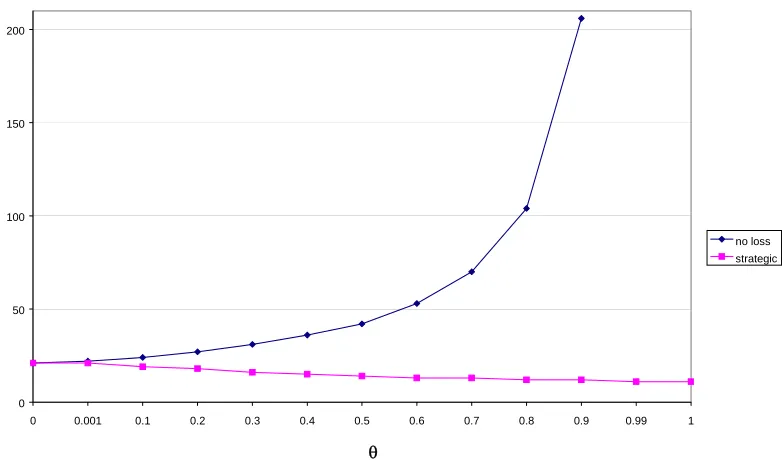
Figure I illustrates Proposition #1 and #2 simultaneously by looking at the relationship
between t* and θ with different initial cost differences, δ. Although in both cases t*
increases with θ (Proposition 1), in the case with a higher initial disadvantage for the
learning firm (δ=.5), t* is higher for each value of θ. We do not include in Fig. I the plot for
θ = 1 or θ = .99 because, as indicated in Table I and II, in the former the learning firm never
emerges, and in the latter it is so large that it distorts the graph (t*= 4149 for δ=.5 and
t*=659 for δ=.4). Each θ represents a unique s* (Table I, column 2). A similar figure could
have been drawn for the case with different N and λ.
It is worth noting that in Table I and II t* seems rather large in many cases. The
values of λ which we are using are drawn from the empirical literature describing annual
learning rates, θ is unit free, while one unit of N could describe any multiple of a basic
product unit. This gives one an inclination to interpret t* as measuring “years” and, supposing
this to be reasonable, Table I paints a rather dire story. Except in the most favourable
circumstances (e.g. N =100, δ≤ .4 and λ = -.5), it might take more than a decade for the new
learning technology to become established (even when selection pressures are not very
severe). In the most unfavourable circumstances (e.g. N =50, δ =.5 and λ = -.1), it might take
as long as 83 years even with a relatively low degree of product market selection (e.g. θ = .5).
Proposition #3: When firm 2 can price strategically, t* decreases in θ, and both
t
0 and T also decrease in θ.The essence of strategic pricing as we have modelled it here is that firm 2 undercuts
firm 1 by an amount ξ. Prior to t*, this generates losses (since firm 2’s costs are higher than
firm 1’s), but these losses are compensated by the profits made after t* when firm 2’s costs
are below firm 1’s costs.7 It takes T periods of profit making after t* for the firm to break
even. Intuitively, it is clear that t* must fall with increases in θ in this case, since a firm that
prices strategically benefits from having price sensitive consumers: the more sales it captures,
the faster it learns. By contrast, in the case of no-loss pricing, firm 2 benefited from having a
relatively high population of noisy consumers in the market, since they are the source of its
sales when it cannot undercut firm 1 (i.e. there is a trade-off between s* and t* with increases
in θ). Recall also that an increase in θ increases s* in all pricing regimes. It follows, then, that
when capital markets allow firm 2 to price strategically, increases in product market selection
pressure unambiguously facilitate the introduction of the new, learning technology: it comes
different relationship between θ and t* under the two pricing regimes, with a given set of
parameters.
FIGURE II
Table III repeats the calculations in Table I with strategic pricing. Columns 3 and 6
indicate the t* which arises with strategic pricing under different initial costs. Comparing
these values to those in columns 3 and 5 in Table I we see that under strategic pricing as θ
increases t* decreases. Columns 4 and 6 show T: the amount of time after t* that it takes the
learning firm to fully pay back its debt accrued by pricing below cost prior to t*. T decreases
as θ increases since the quicker the firm learns the quicker it is able to reach t* and hence
begin making profits to pay back its debt. As with no-loss pricing, increases in N and λ
decrease t* while increases in δ increase t*.
TABLE III
It is interesting to note that capital market selection does not necessarily loosen the
effects of product market selection all that much. If capital markets insist on a pay-back
period of ϕ (meaning that the learning technology only emerges T < ϕ) and if, as seems
casually plausible, this is some number less than 10 years, then Table III indicates that the
learning firm will only be able to payback the loan within that period if it already begins in a
relatively favorable position (low initial cost difference, high learning rate, large market size).
Yet it is precisely in these conditions that the learning firm could have probably gone down
the learning curve quickly enough without the help of capital markets. It is possible to
identify those conditions under which the learning firms should/not take out a loan by looking
example, when there is a 50% initial cost difference, even with low product market selection
θ = .4, the payback period will unlikely satisfy banks (T =30).8 One is tempted to conclude
that while the introduction of capital market selection does in principle facilitate the
introduction of new technologies, in practice relaxation of product market selection pressures
may not have much practical effect.9 This brings us to Proposition # 4 which establishes the
precise conditions under which it is worth it for the learning firm to price strategically (hence
take out a loan).
Proposition #4: The profitability of strategic pricing increases in θ, but no- loss pricing may be more profitable than strategic pricing at low values of θ and when learning is very slow.
Proposition #4 identifies the basic determinants of firm 2’s optimal pricing strategy
conditional on θ, N, λ and δ. The surprising feature of this proposition is that it may pay firm
2 not to price strategically.10 In Table IV and Fig. III we calculate the total profits earned by
the learning firm at t=100 under different parameter conditions.11 Since we know that the
no-loss pricing regime generates neither no-losses nor profits, as long as profits are positive at t=100
we assume it is better for the learning firm to price strategically. To capture changes in the
speed of learning we vary market size but could have shown the same result by varying either
δ or λ.
FIGURE III
We see that when market size is very small (e.g. N=10), no matter what the value of θ
is at t=100, the learning firm makes negative profits (losses) and hence strategic pricing is not
recommended. When market size is intermediate (e.g. N=40) strategic pricing is better only
for values of θ > .4. Only with relatively large market sizes (e.g. N=60-100) is strategic
pricing strategy to pursue under different parameter conditions. The speed of learning is
determined by all three parameters: δ, λ and N.
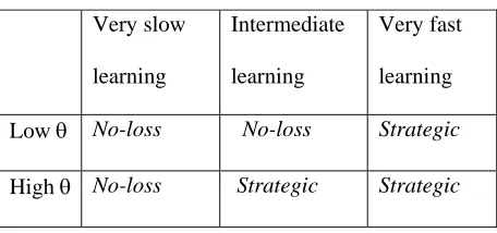
Figure IV: Optimal pricing strategy grid
Very slow
learning
Intermediate
learning
Very fast
learning
Low θ No-loss No-loss Strategic
High θ No-loss Strategic Strategic
Intuitively, this result follows from the observation that no-loss pricing works best
when most consumers are noisy, since the price disadvantage which firm 2 initially suffers is
not penalized when consumers do not care about prices. Hence when θ is low, it is not
necessary for firm 2 to borrow from the capital market to compete. When, in addition,
markets are very small, and/or learning rates are very slow and and/or licensing fees are very
high, then firm 2 will learn so slowly that it will incur a debt that is too large to pay back in an
acceptable time period. When instead firm 2 learns relatively quickly (independent of the
value for θ) and when the degree of consumer price sensitivity is high combined with an
intermediate speed of learning, then it is better for the learning firm to employ strategic
pricing. Hence, strategic pricing brings benefits only when consumers are price sensitive, and
when learning is not too slow (i.e. when N and λ are small and δ is large). This result is of
interest since common intuition might suggest the opposite: it is when learning is very fast
that no-loss pricing might have an advantage since the learning firm could potentially reach t*
relatively quickly even without borrowing.
One of the limitations faced by the model is the simplicity of our specification of
θ, endogenous. This would not only make the demand curve smoother (hence more realistic)
but also allow the pricing strategy employed by firms to evolve with the degree of consumer
price sensitivity. A simple way to make the degree of consumer price sensitivity endogenous
is to postulate that consumers care more about prices the more prices actually differ between
firms (for a homogeneous product). In the no-loss case, this would cause θ to first begin very
high (due to δ), then fall as firm 2 moves down its learning, and then rise again as firm 2
produces past t*. Instead of making price constant in the strategic pricing case, ξ in (4) could
be made to decrease as c2falls (the lower is firm 2’s cost, the more it can afford to undercut
firm 1’s price). Since our results in proposition #4 show that the optimal pricing strategy
depends on both θ and the speed of learning, making θ endogenous would cause the optimal
pricing strategy to evolve. This type of feedback could create interesting dynamics to be
explored via simulation. Nevertheless, our exploration with endogenous θ indicates that the
only real difference is that unlike in the comparative statics excercises with an exogenous θ,
there is no longer a unique s* since s* depends on the value of θ at each time period and
hence at the particular time period market shares are observed. Increases in the speed of
learning cause s* to increase but all the dynamics relating to t* in propositions 1-4 do not
change.12
V. CONCLUSIONS
Studies addressing reasons why best practice techniques do not always become
dominant have focused on the role of positive feedback and network externalities in causing
inefficient techniques to get ‘locked into’. This occurs due to the processes which block
selection from rewarding higher fitness. Here we have looked at another angle of this issue:
the effect of myopic selection in industrial markets on product market performance. On the
face of it, a simple minded application of the natural selection/market competition analogy
would suggest that firms operating in very competitive product markets would not by very
innovative. In particular, an innovation whose introduction incurs costs in the short run will
be a risky proposition for a firm whose performance is judged only on its current activities.
We have argued, however, that this argument is too simple. In the first place, very
competitive markets reward innovations which somehow make it on the market, and the
rewards are more than commensurate with the importance of the innovation (at least for the
kinds of process which our model describes). More fundamentally, the simple analogy
between natural selection and market competition breaks down. This occurs because firms
typically face two different types of selection pressures13. In addition to normal product
market selection forces (driven by consumer behaviour), firms are also selected by the capital
market which governs the conditions under which they can borrow or raise funds. In our
model, it turns out that these two sets of selection pressures do not reinforce each other.
Instead, capital market selection eases constraints on firms in precisely those circumstances
where they are most constrained by product market selection pressures. The fact that product
market selection is myopic means that successful innovations will be well rewarded, and
these, in turn, are the kinds of innovations which capital market agents are most likely to want
to support. As a consequence, when capital markets are not too myopic, the myopia of
Table I: t* with
λ
=.1 and different initial costs and market sizes
Table II: t* with N=100 , different learning indices and initial costs
1 2 3 4 5 6
δ=.4 δ=.4 δ=.5 δ=.5 θ s* t* N=50 t* N=100 t* N=50 t* N=100
1 0% never never never never
0.99 99.50% 659 230 4149 1932
0.9 95% 66 34 411 206
0.8 90% 34 18 206 104
0.7 85% 23 12 138 70
0.6 80% 18 10 104 53
0.5 75% 15 8 83 42
0.4 70% 12 7 70 36
0.3 65% 11 6 60 31
0.2 60% 10 6 53 27
0.1 55% 9 5 47 24
0.001 50.05% 8 4 42 22
0 50% 7 4 41 21
1
2
3
4
5
θ
s*
λ=.1, δ=.4
λ=.5, δ=.4
λ=.5, δ=.9
1
0% never
never
never
0.99
99.50%
230
5
199
0.9
95%
34
2
21
0.8
90%
18
2
11
0.7
85%
12
2
8
0.6
80%
10
2
6
0.5
75%
8
2
5
0.4
70%
7
2
5
0.3
65%
6
2
4
0.2
60%
6
2
4
0.1
55%
5
2
4
0.001
50.05%
5
2
3
Table III: t* with strategic pricing and N=50,
λ
=.1 and different initial costs (
δ
)
Table IV:
θ
vs. profits (
π
) under strategic pricing with different market sizes
(N),
λ
=-.1 and
δ
= .5 (numerical values for Figure III)
1 2 3 4 5 6
N=100 N=60 N=50 N=40 N=10
θ π π π π π
0 139 9.6 -14 -34 -46
0.1 178 26 -3 -27 -48
0.2 218 43 9 -19 -49
0.3 260 62 23 -10 -50
0.4 304 82 37 -0.61 -51
0.5 349 103 53 9.6 -52
0.6 396 124 69 20 -53
0.7 444 147 85 31 -53
0.8 493 170 103 43 -54
0.9 543 194 121 56 -54
1 595 218 139 70 -54
1 2 3 4 5 6
δ=.4 δ=.4 δ=.5 δ=.5 θ s* t* T t* T
1 0% 4 3 21 34
0.99 99.50% 4 3 21 35
0.9 95% 4 4 22 36
0.8 90% 4 4 23 39
0.7 65% 4 5 25 41
0.6 80% 5 5 26 44
0.5 75% 5 5 28 47
0.4 70% 5 6 30 50
0.3 65% 6 6 32 55
0.2 60% 6 7 35 59
0.1 55% 6 9 38 65
0.001 50% 7 9 41 72
Figure I: effect of initial cost difference on t*, with:
λ
=-.1, N=50
Figure II: relationship between t* and
θ
under different pricing strategies
(N=100,
λ
=.1, and
δ
=.5)
0 50 100 150 200 1 0.99 0.9 0.8 0.7 0.6 0.5 0.4 0.3 0.2 0.1 0.001 0 θ t* no loss strategic 0 50 100 150 200 250 300 350 400 450 1 0.9 0.8 0.7 0.6 0.5 0.4 0.3 0.2 0.1 0 theta
t* 40% t*
Figure III:
θ
vs. profits (
π
) under strategic pricing with
different market sizes (N),
λ
=-.1 and
δ
= .5
-100 0 100 200 300 400 500 600
0 0.1 0.2 0.3 0.4 0.5 0.6 0.7 0.8 0.9 1
θ
total profits (
π) N=100
NOTES
1Empirical estimates of learning curves often produce estimates in the region of a 25-30% progress ratio. For example, the B-29 bomber have a progress ratio of 29.5% and large-scale integrated circuits 20% (Scherer and Ross, 1990, p. 98; see also Asher, 1956; Boston Consulting Group, 1972).
2See, for example, Silverberg et al. (1988) and Metcalfe (1997).
3For simplicity, we neglect discounting. Clearly, the higher is the discount rate, the longer it will take to pay back any initially incurred loss caused by investments in learning.
4For more general treatments of optimal pricing when learning by doing is present, see Cabral and Riordan (1994) and Spence (1981).
5Notice that we are not allowing firm 1 to borrow in order to match firm 2’s strategic
pricing. The only possible way that firm 1 could generate future profits to offset current losses incurred in this way would be if it were able to drive firm 2 (and all subsequent entrants) out of the market, and set monopoly prices. However, once it tries to do this, firm 2 can re-enter and begin learning. In the absence of a long run permanent cost advantage over firm 2, it is hard to see how it would be in firm 1’s advantage to prey on firm 2 in this way.
6
This result is also reported by Cabral and Riordan (1994) who observe that the higher is the variance of the distribution of consumer tastes, the higher is the market share of the learning firm.
7Recall that the special structure of the demand function that we are using mean that all that matters is whether firm 1’s price is above or below firm 2’s: the amount of extra sales that the low price firm gets depends only on the fact that it has a lower price and not on the size of the price difference. With more subtle characterizations of demand, the optimal discount (prior to t*) and mark-up (after t*) become interesting choice variables.
8Notice that the introduction of any amount of discounting would increase both t* and
T, making the introduction of the learning technology even less likely.
9
This is, of course, consistent with a large but not always satisfactory literature which asserts that many capital markets (and particularly those in the US and the UK) suffer from “short-termism”.
10For example
, Cabral and Riordan (1994) argue that it is always better for the learning firm to price strategically.
12
In those excercises, we used Eq. (5) below to explore endogenous θ:
{
1 2}
1 (1 ) p p
t
t =γθ− + −γ −
θ where 0≤
γ
≤1 (5)where if γ is close to 0 consumers’ degree of price sensitivity (θ) evolves with price differences and the higher is the price difference the more θ changes, while if γ is close to 1 price sensitivity does not change much.
13
This is also true for the reasons identified in Gould and Lewontin (1979): evolution is not always progressive (fitness enhancing) due to the existence of inertia, non-linearities and random mutations.
REFERENCES
ARTHUR, B. (1989),”Competing Technologies, Increasing Returns, and Lock-In by Historical Small Events,” Economic Journal, 99: 116-131.
CABRAL, L. and M. RIORDAN (1994) “The Learning Curve, Market Dominance and Predatory Pricing”, Econometrica, 62, 1115-1140.
COWAN, R., W. COWAN, and P. SWANN (1997), “A Model of Demand with Interactions Among Consumers”, International Journal of Industrial Organization, Vol. 15: 711-732
DAVID, P. (1985), “Clio and the economics of QWERTY,” American Economic
Review, 75: 332-337.
FOSTER, J. (1993), “Economics and the Self-Organization Approach: Alfred Marshall Revisited”, Economic Journal, Vol. 103: 975-991.
FRIEDMAN, M. (1953), “The Methodology of Positive Economics”, in Essays in Positive Economics, University of Chicago Press, Chicago, IL.
GOULD, S. J. and R.C. LEWONTIN (1979), “The Spandrels of San Marco and the Panglossian paradigm: A critique of the adaptationist paradigm” Proc. R. Soc.,
London B 205: 581-598
GOULD, S. J. (1989), Wonderful Life, Harvard University Press, Cambridge, MA.
METCALFE, S. (1998) Evolutionary Economics and creative Destruction, Routledge, London.
SILVERBERG, G., and G. DOSI, and L. ORSENIGO (1988), “Innovation, Diversity and Diffusion: A Self-Organizing Model,” Economic Journal, 98(393):
SPENCE, m. (1981), “The Learning Curve and Competition,” Bell Journal of
Economics, 12: 49-70.