Wheel Force Sensor Based Techniques for Lose Detection and Analysis of the
Special Road
Huawen Yan 1, Weigong Zhang 2,* and Dong Wang 3
1 School of Instrument Science and Engineering, Southeast University, Nanjing 210096, China; [email protected]
2 School of Instrument Science and Engineering, Southeast University, Nanjing 210096, China; [email protected]
3 School of Instrument Science and Engineering, Southeast University, Nanjing 210096, China; [email protected]
* Correspondence: [email protected]; Tel.:(+86)13809031886
Abstracts: Automobile proving ground is important for the research of vehicles which is used for the vehicle
dynamics, durability testing, braking testing, etc. However, the roads in automobile proving ground will inevitably be damaged with the extension of the service life. In most previous researches, equipment similar to laser cross-section was used to detect pavement quality, the principle of which was to reflect pavement quality by detecting road surface roughness. This method ignores the elastic deformation of the roads itself when the vehicle is traveling on it and hardly compensate for the amendment. Therefore, this article presents a new method based on force sensor to reduce the impact of elastic deformation such as wheel tyre deformation, pavement deformation, and wheel rim deformation. In which, force sensors mounted on the wheels collect the three-dimensional dynamic load of the wheel.The presented method has been tested with two sets of cobblestone road load data, andthe results show that The incentives imposed by the test vehicle on the target road are 88.3%, 91.0%, and 92.05% of the incentives imposed by the test vehicle on the standard road in three dimensions, respectively. It is clear that the proposed method has strong potential effectiveness to be applied for lose detection of the special road application.
Keywords: wheel force sensor, WFS, automobile proving ground, special road, dynamic detection.
1.Introduction
The prototype test is a key part to develop a new car, which is responsible for detecting the presence of defects in the previous part, and test out some of the important performance of the car, such as power, reliability, ride comfort, handling and durability and so on. For example, reference[1]proposes a new anti-lock braking system (ABS) for electric vehicles using visual load, and a sliding-mode controller is proposed for regulating the slip ratio to reach the ideal value for road adhesion; Reference[2]presents an detection damage location of beam structures method based on mode shape extracted from dynamic load of the vehicle to reduce the impact of external environment, the presented method has been tested with experiments, and the results show that the accuracy of location can be reached over 97%; Road load is widely used in automotive durability testing, in order to achieve the durability of the entire vehicle, it is necessary for the entire vehicle, system, subsystem and parts to meet their respective durability requirements[3]; Automobile operational stability is also closely related to the road load, the main test items are: low-speed steering and portable test, steady-state steering characteristic test, transient yaw response test, automotive return-to-negative capability test, steering wheel angle pulse test, steering wheel intermediate position manipulation stability test, etc.[4]; A key factor in the test of automobile fatigue life is accurate acquisition of the random load imposed on the tested item[5]. Mass production is impossible unless the prototype test has achieved a complete success.
The special roads test in the automobile proving ground is an important part of the prototype test, which including cobblestone road test, wash plate road test, gravel road test, wave road test, Belgium road test, twisted road test, pit road test, stone road test, muddy road test and so on, some of the special roads are shown in Figure 1. Different
© 2018 by the author(s). Distributed under a Creative Commons CC BY license.
special road gives the vehicle different frequency and different strength loads, and focusing on different aspects of performance testing. As the extension in road service life, the roads inevitably will be damaged. Traditionally, equipment such as level meter-bar, multi-wheel measuring horizontal vehicle, accumulative jolt instrument, TML high speed pavement meter, GMR pavement meter, and laser cross-section are used to evaluate pavement quality.
(a) (b) (c) (d)
(e) (f) (g) (h)
Figure 1. The special roads: (a)Belgium road; (b) Cobblestone road; (c)Square pit road; (d)Twisted road;
(e) Muddy road; (f) Gravel road; (g)Round pit road; (h)Stone road test.
The principle of level meter-bar is to establish a fixed and non-vibrating reference and measure the deviation between the road surface and the reference [6]. The principle of multi-wheel measuring horizontal vehicle is similar to that of level meter-bar, but its reference is mounted on the supporting wheel of multi-wheel measuring horizontal vehicle to achieve continuous measurement[7]. the accumulative jolt instrument is a mechanical vibration system that runs on the measured road at a certain speed, and its measurement method is indirect measurement[8]. The TML high speed pavement meter is to find the next road surface data by recursive method based on the known road surface data and measurement parameters[9]. The GMR pavement meter based on the inertial reference can directly measure the height difference of the road surface[10]. The laser cross-section is directly measured by a laser sensor installed in front of the vehicle [11]. According to all the above documents, their core principle is evaluated by pavement roughness. Those methods assessing the road grade by road traffic department ignores the road and vehicle interaction process, because the road itself will produce elastic deformation while the vehicles pass the road, and the deformation affect the accuracy of the roughness. We know that the purpose of the special roads is to provide sufficient loads to speed up the testing of the vehicle, which is essentially different from the quality of the rated grade road, and thus there are inherent limitations in the assessment of the special road. Therefore, this paper presents a new evaluation method based on wheel force sensor (WFS), which can accurately obtain the loads applied to the road by the vehicle, and then evaluate the road quality by the statistical analysis of the loads. This approach takes the interaction between the vehicle and the road into account, which is more comprehensive than the methods of evaluating the road’s geometric dimensions alone. WFS is a high-accuracy, 6-axis wheel force measurement system for real-time measurement of forces (Fx, Fy, Fz) and moments (Mx, My, Mz) acting on the wheel hub under dynamic conditions[12]. now some commercial WFS are available, including the 5400 series multiple-axis WFS(PCB Group), the LW series six-dimensional WFS(Kistler Group, Switzerland), SWIFT(MTS Systems Corporation) and the SLW-NC WFS(Tokyo Sokki Kenkyojo Co., Ltd). They have all been applied in many vehicle applications and have acquired acceptable performances[13], however, the application of WFS in road evaluation has rarely occurred. This article uses a three-dimensional force sensor acquisition system developed by Southeast University to achieve the special road lose
detection and analysis, which has a pioneering significance and aims to overcome the problem of dynamic distortion that traditional methods cannot avoid. The WFS is mounted on the axle and rotates with the wheel to dynamically measure the load applied to the road by the vehicle, and the multi-dimensional force sensor measures the force of the wheel in the three-dimensional direction.
2.Materials and Methods
2.1.The principle of road load acquisition
While a vehicle is on the road, because of the effect of the road, the forces on the three dimensions are applied to the wheel, namely the longitude force Fx, the lateral force Fy and the vertical force Fz[14], as shown in Figure 2(a). It is generally known that the role of force is mutual, so the wheel force is equivalent to the road load, in other words, the three-dimensional force of the wheel is equal to the three-dimensional dynamic load of the road. The WFS is attached to the wheel and rotates with the wheel so that real-time acquisition of the dynamic load of the wheel can be achieved. The core principle of WFS is using the strain gauge elastic beams to achieve the force acquisition. Figure 2(b)and Figure 2(c) are the structural and physical views of the 8-beam WFS respectively.
Fy Fz
Fx
(a) (b) (c)
Figure 2. (a) Forces diagram; (b)Diagram of the strain gauge arrangement; (c) Wheel force sensor
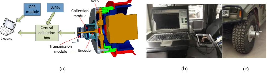
2.2.Road load acquisition system
WFS road load acquisition system is data acquisition system with wheel force sensor as the core and vehicle as the platform. Its block diagram is shown in Figure 3(a), and Figure 3(b)and Figure 3(c) are the upper computer part and the lower computer part of it respectively. The hardware components of the system include WFS, collection module, encoder, transmission module, central collection box, GPS module and laptop. The WFS is connected to the hub of the wheel by customizing the flange plate and enables the collection of road loads in the form of elastic deformation.When the vehicle is running on a road, the wheel and the WFS connected to it simultaneously perform rotational and translational motions, while the body only performs translational motion. This brings two problems:The first is how to send the elastic deformation signal collected by the rotating WFS to the upper computer in the car stably and quickly; The second is how to separate highly coupled x-axis signals and z-axis signals.
Central collection
box
Laptop
Laptop
Transmission module
Collection module
WFS
Encoder WFSs
GPS module
(a) (b) (c)
Figure 3. (a) The diagram of the WFS System; (b) The upper computer of WFS; (c) The lower computer of WFS
In order to solve these two problems, Bluetooth wireless transmission module and angle code disk were introduced. The Bluetooth wireless module is responsible for transmitting the rotating WFS signal to the relatively stationary upper computer, while the angle encoder is responsible for solving the problems of the x-axis and z-axis interaction. The WFS signals and angle signals of each wheel are sent to the central collection box through the collection module and transmission module, and finally sent to the upper computer through the network cable. In the upper computer software, the WFS signal and the GPS vehicle speed signal are further analyzed, processed and displayed synchronously by the data analysis software.
The WFS system is a vehicle-to-road coupling system, so the measured road load is related to multiple factors, which include road type, vehicle type, speed, tire pressure and so on. Road load of different road is not the same, which is the reason for setting various special roads. Different vehicles have different suspension types and weights, and their loads on the road are naturally different. In addition, the impact of speed and tire pressure on road loads is also evident. The vehicle used in this experiment is the military active off-road vehicle, which total weight is equal to curb weight plus weight of testers and equipment for the 3.7t, and the tire pressure was adjusted to 2.7Kg / cm2, the vehicle with WFS system and the type with WFS are shown in Figure 4.
(a) (b) (c)
Figure 4. (a)The diagram of the tyre with WFS, (b) The vehicle with WFS system , (c) The rim with WFS
The sensors in the WFS system are mounted on the left and right wheels of the front axle. The special road used in the experiment was the cobblestone road, which includes a standard road and a target road. The speed of the vehicle is maintained at 40km / h. The original loads data collected by the WFS on the standard road are shown in Figure 5. (a), (b), and (c) of it respectively represent the three-dimensional loads Fx, Fy, and Fz of the left WFS, and (d), (e), and (f) respectively represent the three-dimensional loads Fx, Fy, and Fz of the right WFS. This standard cobblestone road is 200 meters long. When the test vehicle passes at a speed of 40km/h, approximately 5000 effective points are collected. From figures (a) and (d), it can be seen that the driving force Fx is about 2000N. From figures (b) and (e), it can be seen that the lateral force Fy is about 0N. From figures (e) and (f), it can be seen that the vertical force Fz is about 10 thousand N.
(a) (b) (c)
0 1000 2000 3000 4000 5000 6000 7000 -4000 -2000 0 2000 4000 6000 8000
10000 Fx of Left WFT
Sampling point
U
in
t:
N
0 1000 2000 3000 4000 5000 6000 7000 -4000 -3000 -2000 -1000 0 1000 2000 3000 4000
Fy of Left WFT
Sampling point
U
in
t:
N
0 1000 2000 3000 4000 5000 6000 7000 -5000 0 5000 10000 15000 20000
Fz of Left WFT
Sampling point
U
in
t:
N
0 1000 2000 3000 4000 5000 6000 7000 -8000 -6000 -4000 -2000 0 2000 4000 6000 8000 10000
Fx of right WFT
Sampling point
U
in
t:
N
0 1000 2000 3000 4000 5000 6000 7000 -4000 -3000 -2000 -1000 0 1000 2000 3000 4000
Fy of right WFT
Sampling point
U
in
t:
N
0 1000 2000 3000 4000 5000 6000 7000 0.4 0.6 0.8 1 1.2 1.4 1.6 1.8
2x 10⁴ Fz of riht WFT
Sampling point
U
in
t:
N
(d) (e) (f)
Figure 5. The original loads on the standard road, (a)Fx of the left WFS, (b)Fy of the left WFS, (c)Fz of the left WFS,
(d)Fx of the right WFS, (e)Fy of the right WFS, (f)Fz of the right WFS.
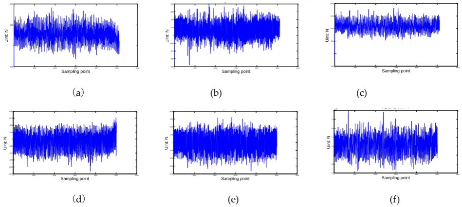
The original loads data collected by the WFS on the target road are shown in Figure 6. Similar to Figure 5, (a), (b), and (c) of Figure 6 respectively represent the three-dimensional loads Fx, Fy, and Fz of the left WFS, and (d), (e), and (f) respectively represent the three-dimensional loads Fx, Fy, and Fz of the right WFS. And the target cobblestone road is also 200 meters long. Similar to the standard road, approximately 5000 effective points are collected. From figures (a) and (d), it can be seen that the driving force Fx is about 2000N. From figures (b) and (e), it can be seen that the lateral force Fy is about 0N. From figures (e) and (f), it can be seen that the vertical force Fz is about 10000 N. Comparing Figure 5 and Figure 6, it is found that the data of the three-dimensional load has a small difference, and it is difficult to find the essential differences between the two roads on the incentive of the test vehicle.Though the difference of original loads between the standard road and the target road is not easy to distinguish from the curve form, but it is difficult to quantify the damage degree of the target road. However, if these incentives are quantified by suitable methods, it is easy to see the degree of wear of the target road. The suitable method used in this paper is the rainflow-counting method.
(a) (b) (c)
(d) (e) (f)
Figure 6. The original loads on the target road, (a)Fx of the left WFS, (b)Fy of the left WFS, (c)Fz of the left WFS, (d)Fx of the right WFS, (e)Fy of the right WFS, (f)Fz of the right WFS.
2.3.Road load processing for rainflow-counting method
In order to cope with the quantification problem, a widely used in the fatigue life calculation rain-flow counting method is introduced. The rainflow-counting method is used in the analysis of fatigue data in order to reduce a spectrum of varying stress into a set of simple stress reversals[15]. Its importance is that it allows the application of Miner’s rule in order to assess the fatigue life of a structure subject to complex loading[16]. The process of counting the load by rain-flow counting method reflects the memory characteristics of the material and has a clear mechanical concept, so the method has been widely used[17]. The basic counting rules are as follows:
The rain flows down the slope from the inside of the peak (valley) value of the load - time series;
A: Stop flowing when the absolute value of peak (valley) value is greater than the one of the initial peak (valley) value;
B: Stop flowing when encountering the above-mentioned rain;
Removing all the full cycles and writing down the valley and peak values for each cycle;
0 1000 2000 3000 4000 5000 6000 -5000
0 5000 10000
Fx of Left WFT
Sampling point
U
in
t:
N
0 1000 2000 3000 4000 5000 6000 -4000 -3000 -2000 -1000 0 1000 2000 3000 4000
Fy of Left WFT
Sampling point
U
in
t:
N
0 1000 2000 3000 4000 5000 6000 -5000 0 5000 10000 15000 20000
Fz of Left WFT
Sampling point
U
in
t:
N
0 1000 2000 3000 4000 5000 6000 -10000 -8000 -6000 -4000 -2000 0 2000 4000 6000
8000 Fx of right WFT
Sampling point
U
in
t:
N
0 1000 2000 3000 4000 5000 6000 -4000 -3000 -2000 -1000 0 1000 2000 3000
4000 Fy of right WFT
Sampling point
U
in
t:
N
0 1000 2000 3000 4000 5000 6000 0.6 0.8 1 1.2 1.4 1.6 1.8
2x 10⁴ Fz of riht WFT
Sampling point
U
in
t:
N
After the first stage of the counting will leave a divergent convergence load-time series, and converting it into a convergent-divergence of the load-time series, and then starting the second stage of the counting until the all of loads are counted. An example is shown in Figure 7.
(a) (b)
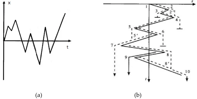
Figure 7. Rain flow counting principle schematic diagram. (a) A sequence of random load data, (b) Clockwise rotation of 90 degrees of random load data.
A random load sequence is shown in Figure 7(a). The first step is to rotate it clockwise 90 degrees to get Figure 7(b). The rain flow method starts at tensile peak 1, which is considered to be the minimum value. The rain flows to peak 2, drops vertically to 2’ between tensile peak 3 and 4, then flows to tensile peak 4, and finally stops at the corresponding point of more negative peak 5 than earlier peak 1, getting a half cycles from 1 to 4 . The next rain flow begins at peak 2 and flows through 3, stopping at the opposite of 4, because 4 is a greater maximum than the starting 2, resulting in a half-cycle 2-3. The third flow starts at the peak 3, because it encounters the rain flow from 2, so it ends at 2’, and getting a half cycle of 3-2’. In this way, 3-2 and 2-3 form a closed stress-strain loop, that is configured as a complete loop 2'-3-2. The 4th flow starts from the peak 4 and passes through the peak 5, dropping vertically to 5’ between 6 and 7, continuing to flow downwards, and then dropping from 7 vertically to the opposite of the peak 10, since peak 10 has a greater maximum value than peak 4, half cycles 4-5-7 are derived. The 5th flow starts from the peak 5, flows to the peak 6, drops vertically, and ends at the opposite of 7, because peak 7 have more negative minima than peak 5. Then take out half cycle 5-6. The 6th flow starts at the peak 6 and ends at 5ˊ because it encounters raindrops from the peak 5 outflow. Half cycles 6-5 and 5-6 are combined into a complete cycle of 5ˊ-6-5. The 7th flow starts at the peak 7 and goes through the peak 8 and falls to the 8’ on the 9-10 line. Then it goes to the last peak 10 and takes out the semicircle 7-8-10. The 8th flow starts from the peak 8 and ends on the opposite side where the flow drops to 9 down to 10 because the peak 10 has a more positive value than 8 and half cycles 8-9 are taken out. The last flow started at a peak of 9 because it encountered a rain drop from a peak of 8, so it ended at 8’. Half-cycle 9-8’ are obtained and paired with 8-9 to form a complete cycle of 8-9-8’. Thus, the strain-time record shown in Figure7(b) includes three full-cycle 8-9-8ˊ, 2-3-2ˊ, 5-6-5ˊ, and three
half-cycles 1-2-4, 4-5-7, 7-8-10 [18].
i=0 j=1 F(0)=E(0)
i=i+1
F(j)=E(i) j = j+1_ E(i)≠E(i-1)
Y
N
f=0 j=j+1 a = E(i+1)-E(i) b = E(i-1)-E(i)
f=f+1 j=j-2 a≥b&b<c
Y
N c = 0
c = b
F(j)=E(i)
(a) (b)
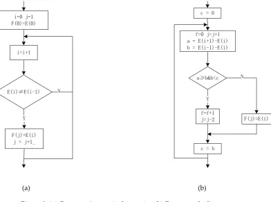
Figure 8. (a) Compression equivalent point, (b) Extract cycle diagram.
It is easy to know that the rainflow-counting method is very suitable for computer programming from the above counting rules. Figure 8 shows how the rainflow-counting method is implemented in the program. It includes two steps: data compression and cycle number extraction. Data compression program flow diagram shown in Figure 8(a). Set the array to be processed to E(n) and the resulting array to F(n). i and j are the numbers of two array elements, respectively. In the compression of adjacent equivalence numbers, the diamond's judgment condition is whether the adjacent two elements are not equal. If it is true, the number is left, otherwise the judgment of the next number will continue until the last number. This removes the first number when it encounters an equal number. The rainflow-counting is to extract the cycle from the compressed data and record its characteristic values such as peak, valley and amplitude. The four-point method that is easier to implement is used in the program. The specific implementation method is shown in flow figure 8(b). In the flow chart, the initial setting of c=0 and the following c=b are some optimizations for the program. The four-point method actually uses only three points. This puts the last calculated E(i-1)-E(i) as the current E(i-1)-E(i-2). s is a flag of whether or not there is a loop. It can be judged whether or not a s is equal to 0 in Figure 8(b). If it is equal to 0, it means that all the loop counts are obtained, otherwise, the entire process of Figure 8(b) will continue to be executed. s is the total number of recording cycles.
3.
Results
The original load data collected by the WFS are input to the rainflow-counting program, and results of the rain-flow matrix are shown in Figure9 and Figure10.
(a)
(b) (c)
(d) (e) (f)
Figure9. Rain-flow matrix of load on the standard road. (a)Rain-flow matrix of Fx on the left WFS , (b)Rain-flow matrix of Fy on the left WFS, (c)Rain-flow matrix of Fz on the left WFS, (d)Rain-flow matrix of Fx on the right WFS , (e)Rain-flow matrix of Fy on the right WFS, (f)Rain-flow matrix of Fz on the right WFS.
(a) (b) (c)
(d) (e) (f)
Figure10. Rain-flow matrix of load on the target road. (a)Rain-flow matrix of Fx on the left WFS , (b)Rain-flow matrix of Fy on the left WFS, (c)Rain-flow matrix of Fz on the left WFS, (d)Rain-flow matrix of Fx on the right WFS , (e)Rain-flow matrix of Fy on the right WFS, (f)Rain-flow matrix of Fz on the right WFS.
The analysis of the rain-flow matrix of load on the target road(Figure10) is similar to the standard road(Figure9), which is also put the original load data in the rain-flow program for obtaining the corresponding rain-flow matrix. The x and y axes of the rainflow matrix are the cycle count of the amplitude and the cycle count of the mean, respectively. Through the comparison between Figure 9 and Figure 10, it can be clearly seen that the standard road has more incentives for the test vehicle than the target road.The reason is that the target road has lost during service. The road load can be quantitatively analyzed after the previous processing, which is also the core value of rain-flow method. Figure9(a) and Figure9(d) are the rain-flow matrix of traction force Fx of the WFS on the standard road. It can be seen
from Figure9(a) and Figure9(d) that the number of rain cycles of Fx is mostly concentrated in about 2000N, which is consistent with the original load in Figure5(a) and Figure5(d) . However, specific quantitative data can be obtained in the rain flow matrix. Similarly, Figure9(b) and Figure9(e) reflect that the number of lateral force rain flow cycles is mainly around 0N, and Figure9(c) and Figure9(f) reflect the number of vertical force rain cycles mainly concentrated near 1.1KN, which also are consistent with the original load in Figure5. In order to do a further description, it is possible to choose any side WFS and the load of any dimension. So the vertical load (Fz) on the left WFS was selected in this paper. The mean value of the Fz of the standard cobblestone road and the target cobblestone road is shown are as in Figure11, and the amplitudes value of the Fz of the standard cobblestone road and the old cobblestone road are shown as in Figure12. It can be seen from Figure11 that the mean value of Fz is mainly concentrated on a quarter of the car’s weight. And the effect on the standard cobblestone road and the target cobblestone road is no significant difference, which is consistent with the car weight is consistent. It is easy to see that the amplitudes value is obviously different from Figure12. The amplitudes value under 2000N of the standard road and the old road are relatively abundant, while the number of load cycles between in 2000N to 4000N is not the same. The target road is clearly less than the standard one, which shows there is consumption about the target road, and it hardly provide enough loads of this level.
(a) (b)
Figure11. The mean value of the Fz, (a) On the standard road, (b)On the target road.
(a) (b)
Figure 12.The amplitudes value of the Fz, (a)On the standard road, (b) On the target road.
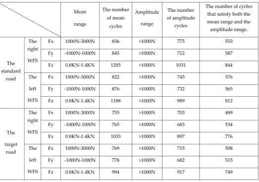
A more detailed description is shown in Table 1, which is rain flow counts after quantification of each dimension load. The theory of fatigue damage accumulation states that when the stress on a part exceeds the fatigue limit, each load cycle causes a certain amount of damage to the part, and this damage can accumulate; when the damage
0.7 0.8 0.9 1 1.1 1.2 1.3 1.4 1.5 x 10⁴ 0 5 10 15 20 25 30 35 40 45 50
Histogram of "rainflow" cycles mean value
N r o f c y c le s : 5 8 7 .5 ( 9 .5 f ro m h a lf -c y c le s )
0.6 0.8 1 1.2 1.4 1.6 1.8 x 10⁴
0 10 20 30 40 50 60 70 80 90
Histogram of "rainflow" cycles mean value
N r o f c y c le s : 8 4 7 .5 ( 4 .5 f ro m h a lf -c y c le s )
0 1000 2000 3000 4000 5000 6000 0 10 20 30 40 50 60 70 80 90 100
Histogram of "rainflow" amplitudes
N r o f c y c le s : 5 8 7 .5 ( 9 .5 f ro m h a lf -c y c le s )
0 1000 2000 3000 4000 5000 6000 7000 0 20 40 60 80 100 120 140 160 180
Histogram of "rainflow" amplitudes
N r o f c y c le s : 4 6 8 .5 ( 5 .5 f ro m h a lf -c y c le s )
accumulates to a critical value, the part will fatigue failure. The linear fatigue damage accumulation theory holds that the fatigue damage generated by each cycle load is independent of each other, so the total damage is the linear accumulation of each fatigue damage[19]. According to the linear fatigue damage accumulation theory, the three dimensions of the WFS load can be arranged as follows: (1) Since the load amplitude of too small has no effect on the fatigue damage of the road, only the number of cycles with a magnitude above 1000 N is calculated in the rain flow matrix.; (2) The number of mean cycles of driving force Fx is mainly concentrated near 2000N, so 1000N to 3000N is taken as the counting range; (3) The number of mean cycles of lateral force Fy is mainly concentrated near 0N, so
-1000N to 1000N is taken as the counting range; (4)The number of mean cycles of vertical force Fz is mainly concentrated near 1.1KN, so 0.8KN to 1.4KN is taken as the counting range.
Table 1. Rain flow counts after quantification of each dimension load.
Mean
range
The number
of mean
cycles
Amplitude
range
The number of amplitude
cycles
The number of cycles that satisfy both the mean range and the
amplitude range.
The standard
road
The right
WFS
Fx 1000N-3000N 836 >1000N 775 553
Fy -1000N-1000N 845 >1000N 712 587
Fz 0.8KN-1.4KN 1205 >1000N 1031 844
The
left
WFS
Fx 1000N-3000N 822 >1000N 745 576
Fy -1000N-1000N 876 >1000N 732 565
Fz 0.8KN-1.4KN 1188 >1000N 989 812
The
target road
The right
WFS
Fx 1000N-3000N 755 >1000N 703 489
Fy -1000N-1000N 765 >1000N 683 534
Fz 0.8KN-1.4KN 1033 >1000N 897 776
The
left
WFS
Fx 1000N-3000N 769 >1000N 715 508
Fy -1000N-1000N 778 >1000N 682 515
Fz 0.8KN-1.4KN 994 >1000N 917 749
Mean and amplitude are two equally important parameters, and the effect of the same load amplitude at different mean levels on the road is not the same. Similarly, different load amplitudes at the same average level also have different effects on the road. Therefore, the number of cycles in the last column of table 1, which is the number of cycles that satisfy both the mean range and the amplitude range, is the core data. Seen from the table, Effective count of the driving force Fx of the right WFS on the standard road and the target road are 553 and 489 respectively, which means
that the target road has less impact on the test vehicle than on the standard road. It is easy to calculate the ratio
Fx_Rbetween two quantified Fx’s, which is equal to 88.4%. Similarly, the following 5 ratios can also be easily obtained,
including
Fx_L=
88
.
2
%
,
Fy_R=
90
.
9
%
,
Fy_L=
91
.
1
%
,
Fz_R=
91.9%
and
Fz_L=
92
.
2
%
. Therefore, Aftersimply averaging the left WFS and right WFS, we can get the ratio of the standard road and the target road in three dimensions as shown in formulas (1), (2)and (3).
%
3
.
88
2
Fx_L Fx_R
Fx
=
+
=
(1)%
0
.
91
2
Fy_L Fy_R
Fy
=
+
=
(2)%
05
.
92
2
Fz_L _R
F
Fz
=
+
=
z(3)
4.
Discussion
According to the existing literature of Wheel force sensor application, researchers are concerned more about the
the research of WFS in the automotive industry, such as dynamics, durability and braking force studies. However, few
people are involved in the application of WFS in road evaluation. In particular, WFS has a unique advantage in the
dynamic evaluation of roads, as compared to traditional road surface roughness evaluation methods.
Based on the above analysis, we present several ways to promote the performance of lose detection and analysis
of the special road in the further study: (1)Multiple road load collection experiment can increase the number of data
sources to improve the stability and reliability of the test; (2) Improved the rainflow-counting model making the calculation process more concise and convenient.
4.1. Multiple road load collection experiment
It is generally considered that the incentive imposed by the special road on the test vehicle is a stationary random
process. Therefore, it is only necessary to collect a set of load data to evaluate a special road according to the ergodic
theory of stationary stochastic processes. However, there are many factors that affect the accuracy of the load data and
cannot be prepared in advance, such as weather, ground humidity and temperature, etc. The load data used in this
article was obtained on a single day. Therefore, it is hoped that multiple seasonal load data can be collected in the
future experiment to eliminate the influence factors mentioned above and make the data as accurate and stable as
possible. In addition, there are all kinds of special roads in the automobile testing grounds, up to 13 kinds. This article
only discusses the special type of cobblestone road, and automobile testing will generally be a combination of several
special types of road testing, Therefore, in the subsequent experiments, all other 12 roads can be assessed to complete
the special road wear detection and analysis of the entire automobile proving ground.
4.2. The rainflow-counting model improvement
The four-peak-valley counting model used in this paper is a traditional calculation model that strictly according to the principle of rain flow counting method. It is the most widely used in practical projects currently. It generally
includes the following 4 steps: (1) data compression; (2) first rain flow count; (3) closure processing of
divergence-convergence data; (4) second rain flow count. It can be seen that the four-peak valley counting model contains two counts of rain flow, and the calculation is complicated. The three-peak-valley count model is based on the four-peak valley count model and is an improvement of the four-peak valley count model. It inherits the basic assumptions such as the closure of the four-peak-valley counting model and its independence from the loading sequence. The three-peak valley counting model guarantees the overall convergence and divergence of data by pre-processing the compressed data, that is, truncating and docking the compressed data, Therefore only one rainflow count is required. Simplifying the calculation process is very critical in real-time processing. This will fully prepare the
WFS system for real-time evaluation of roads based on mobile platforms.
5.
Conclusions
In order to overcome the shortcomings of traditional methods that cannot dynamically evaluate the special roads, a new method of road lose analysis based on WFS is proposed. After completing the assessment of the road with the WFS system, the loads of the special road for each wheel can be quantified. It is clear to know how many loads the standard road or the target road can provide to the vehicle, and after calculation, we can know that the target road provides incentive to the vehicle in traction equivalent to 88.3% that provided by the standard road, and 90.0% and 92.05% of the lateral and vertical forces, respectively. This is a way to analyze the quality of the road from the perspective of the purpose of the special roads, and it reflects the nature of the special roads.
Conflicts of Interest: The authors declare no conflict of interest.
References:
[1]. Lin, C., et al., Antilock braking control system for electric vehicles. The Journal of Engineering, 2018. 2018(2): p. 60-67.
[2]. He, W., J. He and W. Ren, Damage localization of beam structures using mode shape extracted from moving vehicle response. Measurement, 2018. 121: p. 276-285.
[3]. Xu, L., et al., Design of durability test protocol for vehicular fuel cell systems operated in power-follow mode based on statistical results of on-road data. Journal of Power Sources, 2017. 377.
[4]. Li, Z., et al., Parameter sensitivity for tractor lateral stability against Phase I overturn on random road surfaces. Biosystems Engineering, 2016. 150: p. 10-23.
[5]. Yan, D., et al., Fatigue Stress Spectra and Reliability Evaluation of Short- to Medium-Span Bridges under Stochastic and Dynamic Traffic Loads. Journal of Bridge Engineering, 2017. 22(12).
[6]. Hassan, R. and R. Evans, Road roughness characteristics in car and truck wheel tracks. International Journal of Pavement Engineering, 2013. 14(8): p. 736-745.
[7]. Cheng, G., et al., Research on the Airport Pavement Roughness Evaluation Based on Full Aircraft Model. Highway Engineering, 2016.
[8]. Katicha, S.W., J.E. Khoury and G.W. Flintsch, Assessing the effectiveness of probe vehicle acceleration measurements in estimating road roughness. International Journal of Pavement Engineering, 2016. 17(8): p. 698-708.
[9]. Radopoulou, S.C. and I. Brilakis, Automated Detection of Multiple Pavement Defects. Journal of Computing in Civil Engineering, 2016. 31(2): p. 04016057.
[10]. Kim, R.E., et al., Stochastic Analysis of Energy Dissipation of a Half-Car Model on Nondeformable Rough Pavement. Journal of Transportation Engineering Part B Pavements, 2017. 143(4): p. 04017016.
[11]. Alleva, L., ROAD SURFACE ROUGHNESS MEASURING SYSTEM AND METHOD. 2012, WO.
[12]. SD, R.M.A.J., A sensor for measurement of frition coefficient on moving flexible surfaces. IEEE senors, 2005. 5(5): p. 844-849.
[13]. Kim JH, K.D.S.A., Design and analysis of a column type multi-component force/moment sensor. Measurement, 2003. 3(33): p. 213-219.
[14]. Lin, G., et al., A self-decoupled three-axis force sensor for measuring the wheel force. Proceedings of the Institution of Mechanical Engineers, Part D: Journal of Automobile Engineering, 2014. 228(3): p. 319-334.
[15]. Shinde, V., et al., Modified Rainflow Counting Algorithm for Fatigue Life Calculation. 2018.
[16]. Chen, C., et al., Load spectrum generation of machining center based on rainflow counting method. Journal of Vibroengineering, 2017. 19(8).
[17]. Sadowski, N., et al., Evaluation and analysis of iron losses in electrical machines using the rain-flow method. IEEE Transactions on Magnetics, 2000. 36(4): p. 1923-1926.
[18]. Liu, G., D. Wang and Z. Hu. Application of the Rain-flow Counting Method in Fatigue. in International Conference on Electronics, Network and Computer Engineering. 2016.
[19]. Bisping, J.R., et al., Fatigue life assessment for large components based on rainflow counted local strains using the damage domain. International Journal of Fatigue, 2014. 68(11): p. 150-158.