Simulation of saltation motion using LBE based methods

(1)

Simulation of saltation motion using LBE based methods

Jindˇrich Dolansk´y1,a

1_{Institute of Hydrodynamics, ASCR, Pod Paˇtankou 5, Prague, Czech Republic}

Abstract. The numerical model of the motion of the circular particle close to the bed in an open channel with a rugged bed based on the lattice Boltzmann method (LBM) is presented. The LBM is used as a DNS approach in which hydrodynamic forces are expressed as sum of contributions from fluid elements interacting with the moving particle. The corresponding numerical simulation for the saltation motion which represents a dominant mode of the bed load transport is developed. Flow is driven by the logarithmic velocity profile at the inlet of a two dimensional channel with a bed formed by semi-circles of variable radii in a bed of particles. Translational and rotational movements of the particle are induced by gravitational force on one hand, and by hydrodynamic forces on the other hand. The LBE (lattice Boltzmann equation) based simulation provides the opportunity to study the behavior of saltation motion in the moderate and high Reynolds number regimes. Most of the input parameters, including boundary conditions or flow conditions, are adjustable within a range of values. Stability issues of the simulation are considered and a resolution using a combination of different LBE models and the extension of computational resources is proposed. Finally, an enhancement of the simulation for more complex processes is suggested.

1 Introduction

Particle movement influences the flow of the fluid and its trajectory is affected by the flow in return. The influences can be classified within three types of interactions: parti-cles with the fluid, mutual (particle-particle) collisions and particle collisions with the bed (particle-bed). Simulations of particle motions and their interactions close to the bed represent a significant focus recently in hydrodynamics.

Bed load transport is defined as the motion of parti-cles close to the bed which occurs in three different modes: rolling, saltation, and suspension. These modes merge into themselves mutually either in the mentioned or the reversed order depending on flow conditions (shear velocity, fluid density and viscosity), particle attributes (size, shape and density) and bed characteristics (roughness and ruggedness expressed in terms of bed particles size and their respective packing density). As particles within a single cluster differ in shape, size and density, they can move in various modes in the same time.

It has been shown that saltation represents the domi-nant mode of the bed load transport. Saltation is a compli-cated motion of particles which consists of free motion in the ﬂow, mutual collisions of particles and collisions with the bed. The characteristic pattern of the saltation mode is determined mainly by particle-bed collisions.

The lattice Boltzman method (LBM) is a two decade old developed numerical approach originating from the lat-tice gas automata methods used for the simulation of com-plex fluid flows, e.g., [1–3]. LBM represents a second or-der, efficient computational scheme due to its inherent lo-cality and explicitness. Moreover, the possibility of straight-forward parallelization yields another considerable advan-tage of the traditional numerical approaches to fluid flow problems.

a _e-mail:_{[email protected]}

Traditionally, models of saltation are composed from four ingredients: equations for the fluid flow (e.g., Navier-Stokes), equations for motion for particles in the flow (de-rived from Newton laws), impulse equations describing particle-bed collisions and a particle-particle collision model. These equations are then discretized by finite difference or element methods and standard numerical methods are ap-plied to the resulting algebraic equations.

In contrast, LBE methods offer quite a general and ro-bust tool to solve the above mentioned stages of the salta-tion mosalta-tion within a unified frame when it is used as a di-rect numerical simulation (DNS) technique. Particle-fluid systems represent a significant category of applications of the LBE methods that have recently been developed and examined.

The aim of this work is to develop and test a LBE based simulation of the motion of the particle in the flow founded on the mesoscopic – scale between molecular and continu-ous (macroscopic) domain – model of the fluid. The math-ematical model is designed for the saltation motion in an open channel and implemented employing LBM. It is shown that LBM can be equally used to model saltation motion and the resulting simulation produces likely and expectable results in comparison with the traditional approaches men-tioned above without a loss of efficiency of the computa-tions.

From the reason of the initial testing of the LBE based simulation, it is supposed that particle to particle collisions occur quite rarely, and hence it is sufficient to consider the motion of the single particle in the flow. The flow is driven by the logarithmic velocity profile at the inlet of a two di-mensional channel with a bed formed by semi-circles of variable radii in a bed of particles. The saltating particle has a circular shape and it is not deformable. Translational and rotational movements of the particle are induced by gravitational force, and by hydrodynamic forces. The latter DOI: 10.1051/

C

Owned by the authors, published by EDP Sciences, 2014 /2 01

epjconf 4 6 70 2 020

(2)

forces are modeled on the mesoscopic level as interaction between the ﬂuid elements and the particle, see Sect. 3.

The LBE based simulation – after some modiﬁcations, see Sect. 5.2 – enables the chance to study the behavior of saltation motion in the moderate and high Reynolds num-ber regimes. Most of the input parameters including, bound-ary conditions or ﬂow conditions, are adjustable within a range of values.

This paper proceeds as follows. In the next section, the numerical model for ﬂow and particle motion and its colli-sions with the bed are described at the macroscopic level. In Sect. 3 essentials of LBM are introduced. In Sect. 4 the numerical model of the motion of the particle in the ﬂow is implemented in the mesoscpic level, i.e., using the LBE approach. Results and consequent observations are presented in Sect. 5 which consists of graphs demonstrat-ing the outputs of the simulation and stability considera-tions concerning the simulation. Finally, the paper is sum-marized in Sect. 6 where also prospective plans are pro-posed.

2 Numerical model

2.1 Flow ﬁeld

We assume that the ﬂow is determined by the incompress-ible Navier-Stokes equations

ρf

_∂

u

∂t +u· ∇u

=−∇p+μ∇2u,

with constant kinematic viscosityν. We suppose that the mean velocity of the ﬂow is determined by the logarithmic law of the wall

ux=u∗

k ln(

y0

y_u∗) (1)

close to the bed as it can describe ﬂows at higher Reynolds numbers.k = 0.4 stands for the Karman constant,u∗ for shear velocity andy0for the distance from the bed at which the velocity u goes to zero.

The domain of the process is confined within the bound-aries of two types: open boundbound-aries (inlet, outflow and free water surface), and solid boundary (bed). Each boundary is represented by a different boundary condition.

Flow velocity is driven by the logarithmic velocity ﬁle at the inlet of the channel, cf. Eq. (1). The velocity pro-ﬁle is induced long enough to achieve a steady state.

At the outﬂow, the Neumann free ﬂow – the so called “do nothing” – boundary conditions are imposed

−pn+ν∂_∂u_n =0, (2)

which corresponds to the normal gradients of the velocity set to zero (nrepresents the outer normal to the boundary), e.g., [4]. These conditions are often used if any boundary conditions for the velocity at the outﬂow are not prescribed and represent a popular choice for open boundaries for the incompressible Navier-Stokes equations.

As it is supposed that the process takes place in an open channel; the water level is described by a free sur-face boundary condition which is characterized by constant pressure

p(xlevel)=const.

The bed of the channel is composed of half-circles with radii equal to the radius of the saltating particle. The no-slip boundary condition – identiﬁcation of the ﬂuid veloc-ity with the velocveloc-ity of the corresponding surface – is sup-posed on the bed

u(xbed)=0, as well as on the particle surface:

u(xbn)=vtot(xbn),

where the subscript “bn” denotes the boundary nodes of the moving particle.

2.2 Particle motion

The motion of a particle in the ﬂow is determined by ac-tions of both body and hydrodynamic forces. They are summed into a resultant net force F_net which occurs on the right-hand side of the Newton equations

d2x dt2 =

Fnet

m , (3)

and thus determines the particle motion (m=ρpVis mass of the particle). The net force results from the summation of body and surface forces

Fnet=Fg+Fd+Fm+FM+FB, (4)

whereFgstands for gravitational force and hydrodynamic forces are represented by drag forceF_d, force due to added massFm, the Magnus forceFMand the Basset forceFB.

The net force develops a torque on the saltating parti-cle which determines its surface angular velocityωfrom relation

Jdω

dt =r×Fnet,

whereJ is the particle momentum of inertia andris the vector pointing from the center of the particle to a boundary point. It has been shown that rotation influences both mo-tion and collisions significantly, and especially for higher Reynolds particle number, rotation has to be taken into ac-count as it essentially affects particle trajectories [5].

2.3 Particle-bed collision model

Descriptions of particle-bed collisions use to be based on impulse equations which result into relations between ve-locities before and after a collision. If the approach by Ni˜no and Garcia [6] is adopted then

v x= f

v2

x+v2y cos(θin+θb)

cos(θr+θb) cosθr

v

y= f

v2

x+v2y cos(θin+θb)

sin(θr+θb) cosθr

whereθin represents the incidence angle, θb is the angle between the tangent line passing through the contact point and the bed line andθris computed from

tanθr= e

(3)

where e and f represents restitution and friction coeﬃ -cients respectively. Since the bed is irregular – in this case made of circles – a random number generator is used to pick out one location from all possible contact points and thus to determine the angleθb[7].

Rotation has to be taken into account and the particle angular velocity is expressed appropriately. It is supposed that the particle rebounds without the slip in the current phase of development of the simulation. In other words, the bouncing particle does not slip along the surface of the bed during the collision which allows to express the an-gular velocity after collision (also solution of the impulse equations) as

ω₌_ω₋mtot(vt+rω)r J+mtotr2

, (5)

wheremtot represent the sum of the particle massmand the added mass, andvtcorresponds to the tangent velocity component just before the collision, cf. [7].

It should be mentioned that although collisions with the bed determine the characteristic pattern of the saltation motion; particle-particle collisions aﬀect the characteristic parameters of the saltating motion as height and length of jumps or the vertical particle distributions.

However, as in this work the saltation motion of a sin-gle particle is considered, it is not necessary to deﬁne the particle-particle collision model though as it will be in-cluded into the developed simulation.

3 LBM intro

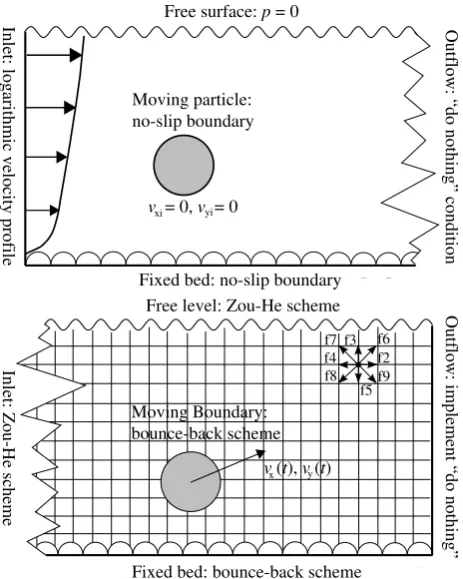
The LBE approach is designed to view flow processes from a mesoscopic (situated in between microscopic and macro-scopic levels) view. Formulation of a numerical model based on the LBE method is determined by postulating meso-scopic structure determined by choice of: (a) a lattice grid specified by space dimension and nodes layout, e.g., quadratic, hexagonal, cubic, (b) a set of discrete velocitiesci connect-ing the nodes, (c) a collision operator Γi for interactions of fluid elements at the nodes and (d) implementation of boundary conditions, cf. figure 1.

Fluid elements that can move only along discrete veloc-itiesci in a selected lattice are represented by distribution functions f(x,ci,t) ≡ fi(x,t) which gives the probability of finding a fluid element in locationxwith a velocity of ciin timet. Collision rules that guarantee conservation of mass and momentum are applied on the fluid elements at grid nodes. The collision and propagation process is repre-sented by the lattice Boltzmann equation

fi(x+ciΔt,t+Δt)−fi(x,t)=Γi. (6) Due to collision; the distribution function fi, aligned in the direction c_i at positionx and time t, is updated with

Γi after which propagates to the position x+ciΔt at the next time stept+Δt. The collision operator expresses the propensity to the local equilibrium feq and it is often ap-proximated by a simpler Bhatnagar-Gross-Krook operator

ΓBGK i =

1

τ(fieq−fi), (7) where change of the distribution function fiis proportional to its diﬀerence from equilibrium feq_{. The parameter}_τ ex-presses the rate of tendency to local equilibrium and it must

be deﬁned so as to imply the desired macroscopic dynam-ics. The equilibrium distribution function feqcorresponds to the Maxwell distribution of molecule velocities

f_ieq=ρwi

1+ciu c2

s

+(ciu)2−c2su2 2c4

s

(8)

which is expanded to the second order in the Mach num-berMa = u/cs where parameterswirepresent weights in directionscinormalized asiwi=1. Hence, the so called collision step

fic(x,t+Δt)=fi(x,t)+ 1

τ(fieq−fi), (9)

represents the collision of ﬂuid elements in a node, or ten-dency of distribution function to the equilibrium distribu-tion (8).

Macroscopic quantities (densityρand velocityu) of the ﬂow are obtained as moments over particle distributions

ρ_f =

i

fi, u=

i

fici. (10)

It can be shown that such a simple collision-propagation scheme leads back – by the method of the asymptotic anal-ysis – to the macroscopic Navier-Stokes equations in the incompressible limit.

From the relations for collision operator (7) and the equilibrium distribution (8) it is evident that the calcula-tion of the post-collision distribucalcula-tions fc

i is localized, i.e., it depends only on the distributions in a node and its direct neighbors. This fact determines the parallel nature of the LBE based methods. Moreover, in the stream step

fi(x+ciΔt,t+Δt)= fic(x,t+Δt), (11)

distributions fi spread along straight lines with constant speedsci(in a chosen lattice). Thus, collision step (9) along with stream step (11) represent a two-step algorithmization of the lattice Boltzmann equation (6).

4 Implementation

4.1 Boundary conditions

The implementation of diﬀerent boundaries types is more or less straightforward within the LBE frame. However, any implementation scheme has to allow passage – by the asymptotic analysis – from a mesoscopic formulation of boundary conditions to their macroscopic counterparts (within certain accuracy limits).

Four boundary conditions mentioned above – open bound-aries of the inlet, outflow and free surface side, and the solid boundary of the bed – require the usage of different imple-mentation techniques. The outline of the process domain along with the boundaries and their implementation is de-picted in figure 1.

The no-slip boundary condition on the solid surface of the bed made of semi-circles – as well as the particle solid surface – is implemented by the so called bounce-back scheme which consists in the inversion of distribu-tions

(4)

Free surface: p = 0

Fixed bed: no-slip boundary

Inlet: logarithmic velocity profile _{Outflow: “do nothing” condition}

Moving particle: no-slip boundary

vxi = 0, v = 0yi

f2 f4

f6

f9 f7

f8 f3

f5 Free level: Zou-He scheme

Fixed bed: bounce-back scheme

Outflow: implement “do nothing”

Inlet: Zou-He scheme

Moving Boundary: bounce-back scheme

v x(t), v y(t)

Figure 1.The saltation motion of the particle in an open channel: Boundary conditions and physical parameters at the macroscopic level are depicted in the upper figure. The D2Q9 implementation of the conditions and lattice distributions fi is illustrated in the lower figure. The grid is actually far more finer with respect to sizes of both moving and bed particles.

along the directions of incident to the boundary nodes. In the case of moving a boundary, the bounced distributions must be modiﬁed

fi(xbn,t+1)= f₋ci(xbn,t)+2wi

ρ(xbn,t) c2

s

(ci·vtot(xbn,t)) (12)

due to the exchange of momentum between ﬂuid elements and the moving particle, cf. Eq. (14), wherev_tot =v+r×ω denotes the total velocity at the boundary nodes. The im-plementations can diﬀer in treatment of the object interior, e.g., [8, 9], or its surface curvature [10].

The specified velocity profile at the inlet is implemented by the Zou-He boundary scheme [11] which allows to de-fine velocityu(xin,t) or pressure p(xin,t) on the boundary. In this case, only the non-equilibrium part of distributions are bounced-back in the normal direction with respect to the boundary

fi−f_ieq= f−i−f₋eq_i,

where indexiruns over only unknown distributions. This assumption helps to express the distributions along with imposing macroscopic velocity/pressure conditions. The same scheme is used to implement the free surface boundary with constant pressure which represents the water level.

The corresponding LBE schema to the “do-nothing” condition given in terms of the hydrodynamical variables, see Eq. (2), is derived with the help of asymptotic analysis

and implemented by two relations

fi(xout,t+1)= f_ieq(xout,t)−

_ν_∗

τ −1

f₋neq_i (xout,t),

for the direction opposite to the outer normal,c_i=−n, and

fi(xout,t+1)=f−ci(xout+ci,t)− 2wi

c2 s

u(xout−n,t)·ci,

for the other directionsci−n, e.g., [12]. The equilibrium distributionf_ieq, see Eq. (8), is deﬁned for constant density

ρ=1 instead of ﬂuctuating density given by Eq. (10). The lattice nodes on which the outﬂow is located are denoted xoutandν∗is the lattice viscosity.

4.2 Particle motion

In the case that LBM is used as a DNS technique, move-ments of an object in the flow is the effect of interaction of fluid elements (represented by distributions fi) with the solid surface of the object. The interaction consists of the action of fluid elements on the particle motion, and the ac-tion of the particle on the fluid elements, i.e., on the flow. The first action moves the particle and is determined by the net forceFnetof the fluid elements, Eq. (13). The second interaction is implemented as a special – moving – case of bounce-back boundary conditions, cf. Eq. (12).

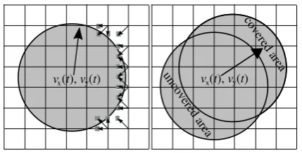
The particle motion is caused by the momentum trans-ferΔpfrom the incident fluid elements. Time rate of this momentum transfer defines the force by which the flow acts on the particle. The net forceFnet which enters the New-ton equation (3) is the sum of the force due to the momen-tum transfer between the particle and fluid elements and the forces due to the nodes covered/uncovered by the particle within time stepΔt

Fnet=Fbn+Fcov+Fun, (13)

cf. ﬁgure 2. As in the macroscopic case, the net force is the sum (4) of particular hydrodynamic forces (drag, added mass, Magnus, Basset etc.).

The momentum contributionΔpforms an impulse force on the particle given by

Fbn=−

Δp

Δ_t =

bn

i 2c₋i

fc

−i(xbn,t)+wi

ρ(xbn,t) c2

s

(ci·vtot(xbn,t))

,

(14) withΔt=1, cf. [9].

The impulse forceFcov exerted on the particle due to covered nodes is given by the momentum sum from the previous time step

Fcov=

cov

i

cifi(xcov,t−1).

Total momentum in uncovered nodes forms the negative impulse force increment

Fun=−

un

ρ(xun,t)u(xun,t),

(5)

v x(t), v y(t) v x(t), v y(t) uncovered area

covered area

Figure 2.The net force which determines particle motion is com-posed of three particular forces. (a) force due to momentum ex-change in the boundary nodes of the particle. (b) forces due to the momentum of ﬂuid elements in nodes covered by the particle and the momentum of uncovered particle nodes.

4.3 Integration of equations of motion

The hydrodynamic forces on the right-hand side of the New-ton equation are the eﬀect of interaction of ﬂuid elements with the moving boundary. To update the particle position (x(t), y(t)) and velocity (vx(t), vy(t)) the left-hand side of the Newton equations has to be evaluated every time step. In other words, a computational procedure for integration of the Newton equations (3) is required.

For this purpose, the leap-frog algorithm is chosen as it is simple, possesses second order accuracy, is invariant un-der time reversal and has other global properties, e.g., it is an area preserving map in phase space when integrating the Newton equation over a ﬁnite time, e.g., [13]. The equation of the motion of the particle can expressed as

dx dt =v,

dv dt =

Fnet

m ,

which are approximated by two (leap-frog) iteration for-mulas

xn+1=xn+Δtvn+1/2 , vn+3/2=vn+1/2+ΔtF(xn+1),

executed every half-time step.

4.4 Conversion into lattice units

To complete implementation of the numerical model, all the physical input quantities describing the ﬂow and the particle have to be converted into their lattice counterpart. It is achieved by setting the conversion factors from the system of physical units (meter and second) into the system of lattice units (lattice unit and time step). These factors result from the relations between physical time and space elements,ΔxandΔt, and lattice time and space elements which are set to equal to unit,Δx∗=Δt∗=1.

If the physical length [L]=m is discretized by a lattice withNnodes then

Δ_x Δx∗ =

L

N m,

for the space element.

The time elementΔtshould not be too small, otherwise it would result in a too small value of the lattice viscosity

ν∗₌_ν Δt

Δ_x2.

Consequently,

τ≡ ν∗ c2 s

+1

2 → 1

2, (15)

and therefore the LBE method becomes unstable because of incapability to dissipate the energy due to very large ve-locity gradients.

The time step Δt can be determined by various ways depending on the speciﬁc model. Namely, it can be deﬁned from ratio of physical and lattice sound velocity

Δt=Δx cs

Cs =

L/Cs N/cs

sec,

or by setting the relaxation parameterτ >0.5 ensuring sta-bility from

Δt=ν Δx 2

c2

s(τ−0.5) sec,

or by assigning a maximal lattice velocity of the ﬂow from relation

Δt=Δx u ∗ max uchar

sec,

with respect to a characteristic macroscopic velocityuchar. Additionally, a requirement on incompressibility

Ma=u∗max/cs1 must be satisﬁed for all cases. It is pos-sible to choose any of the above mentioned conversion meth-od in the simulation.

5 Results and observations

The developed simulation which models the particle mo-tion and the velocity ﬁeld of the ﬂuid is initially expected to reproduce correct physical behavior to demonstrate its capacity to compete with traditional CFD methods.

Most of the input parameters are adjustable within a range of values, e.g., maximal inlet velocityuchar, shear velocityu∗, radius of both the moving particle and the bed particles, density of both the fluid and the particle or phys-ical viscosityν. Such a variability in the physical input pa-rameters leads to good flexibility in modeling various phys-ical conditions of the particle-fluid system.

For the resulting illustrations bellow it is supposed that the process is performed in an open channel of the length L = 1 m and heightL/10 with bed particles of radiirb = L/100. The flow is driven by the logarithmic velocity pro-file with maximal valueu(0,L/10)=0.4 m.s−1_{at the inlet} where the fluid densityρ = 1000 kg.m−3. The kinematic viscosity of water isν=10−6 m2.s−1, but for the stability reasons, see Sect. 5.2, fluid of viscosityν=10−4 _m2_._s−1_is examined. Thus the Reynolds number reduces fromRe = ucharL/ν ≈105 (the particle Reynolds numberRep ≈104) toRe≈103₍_Re

p≈102).

The radius of the moving particle is assumed to be equal to the radii of the bed particles, i.e.,r=rb =L/100. The saltating particle is released in the steady state flow (gen-erated by the inlet logarithmic velocity profile flow) from x0 = L/5 andy0 = L/3 with zero translational and ro-tational initial velocity (vx0, vy0) = (0,0) andω = 0. The process is examined with the sand-like particle of density

(6)

50 100 150 200 250 300 350 400 450 500 20

40 60 80 100

Channel

Height

Length

50 100 150 200 250 300 350 400 450 500

20 40 60 80 100

Channel

Height

Length

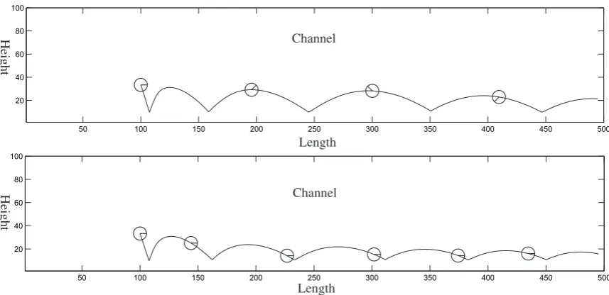
Figure 3.Trajectory of the particle versus length and height of the channel for the rotating and non-rotating-particle. The particle trajec-tories are depicted with respect to the length and height of the channel expressed in lattice space units. It can be seen that rotation around the particle center inﬂuence both length and height of jumps, and also their number within the examined domain. Speciﬁcally, the rotating particle undergoes less of larger jumps in the observed part of the channel.

5.1 Comparison of rotating and non-rotating particle

From comparison of results for rotating and non-rotating particle can be seen how this assumption affects behavior of the saltating particle. Thus, figures below serves as illus-trations of the basic visual outputs of the simulation which are used to characterize the particle motion and the fluid flow.

In the first figure 3 two particle trajectories (x(t), y(t)) are compared corresponding to the rotating and non-rotating particle. The trajectories are depicted with respect to the length and height of the channel expressed in lattice space units. It can be seen that rotation around the particle center influences both length and height of jumps, and also num-ber of jumps within the examined domain. Specifically, the rotating particle undergoes less of larger jumps in the ob-served part of the channel.

The trajectory shapes considered above implies that also translational velocity components (vx(t), vy(t)) differ for both cases. Specially, the rotating particle moves faster in both components of velocity vectorvwhich also results in dif-ferent time spent within the observed domain. Hence, the rotating particle spends in the process domain about one fifth less of lattice time steps with respect to the non-rotating one, cf. figure 4.

For illustration also the angular velocity with respect to the number of lattice time steps is depicted where the colli-sion events can be detected as discontinuous changes in the quantity development. The angular velocity is described by a graph with few jump contributions – determined by change in angular velocity within the collision, cf. Eq. (5) – compensated by successive increase (in absolute value) following after the collision, cf. ﬁgure 5.

The velocity ﬁeld (ux(t),uy(t)) of the ﬂow is driven by

the logarithmic velocity proﬁle at the inlet on one side, and by the interaction of the ﬂow with the moving particle on the other side.

0 500 1000 1500 2000 2500

−0.2 −0.1 0 0.1 0.2 0.3 0.4 0.5

Iteration

v

,

v

components

x

y vy

vx

Figure 4.Velocity components (vx(t), vy(t)) are compared for a

ro-tating or non-roro-tating particle. The characteristic alternating pat-tern can be seen for they-component as the particle undergoes collisions with the bed. The translational velocity components (vx(t), vy(t)) diﬀer for both cases: The rotating particle moves

faster in both components of velocity vectorvwhich also results in diﬀerent time spent within the observed domain. The rotating particle spends in the process domain about one ﬁfth less of lattice time steps with respect to the non-rotating one.

Before the particle is released it behaves as a station-ary solid circular obstacle with two asymmetric eddies (de-termined by the asymmetric initial position of the particle with respect to the height of the channel) separated from the surface of the particle. The eddies maintain themselves till the particle starts to move. Then the eddies start to circle around the particle and deform dramatically.

(7)

veloc-0 500 1000 1500 2000 −0.09

−0.08 −0.07 −0.06 −0.05 −0.04 −0.03 −0.02 −0.01 0

Iteration

Angular velocity

Figure 5.Angular velocity with respect to the number of lattice time steps. The angular velocity is described by a graph which with few jump contributions – determined by change in angu-lar velocity within the collision – compensated by successive in-crease (in absolute value) following after the collision.

ity on the particle surface than in the non-rotating process, cf. ﬁgure 6.

Also the coarse-grained subdivision (discussed after-ward in Sect. 5.2) of the lattice can be detected. Obviously, the proposed reﬁnement of the lattice should introduce more precision into the simulation of the saltation motion and thus enable its signiﬁcant improvement.

5.2 Stability issues

The very low viscosity of water results in high Reynolds numberRe=uL/νregime of the ﬂow. This means that the relaxation parameterτ≈0.5, cf. Eq. (15), and that the sim-ulation becomes potentially unstable. The instability issues are cured in various ways.

Better stability or an increase of the relaxation parame-ter could be achieved by refining the lattice grid. However, the simulation operates currently on a rather coarse-grain lattice with respect to the physical dimensions of the ex-periment because of various reasons. First, the rather coarse grid allows immediate observations of potentially unstable regions in the process domain. Secondly, grid refinement yields significantly increase in demands on computational resources.

This is will be achieved by using the CUDA GPU com-puting technology transformation which can be applied on the Matlab code which takes advantage of the Parallel Com-puting Toolbox. Due to the inherently parallel nature of the lattice Boltzmann it is expected that it will result in a sat-isfactory acceleration of the calculation. Consequently, it enables to reﬁne the lattice grid signiﬁcantly.

Except for the reﬁnement of the grid, the stability prop-erties of the simulation can be improved by modiﬁcations of the LBE model. It is worth to mention the best known LBE based methods for which stability reasons have been developed: regularized, entropic and multi-relaxation time LBM.

The regularized LBM is based on a replacement of the distribution functions by their regularized counterparts which guarantees symmetries resulting from the Chapman-Enskog

expansion, e.g., [14, 15]. The entropic LBM is based on the second thermodynamic law and uses the Boltzmann H-theorem [16, 17]. The multi-relaxation time LBM, e.g., [18], replaces the LBGK collision model Eq. (7) with a multi-relaxation-time collision model which allows adjust-ment relaxation times independently for each of moadjust-ment of distribution, cf. Eqs. (10).

One of the mentioned stabilization techniques, specifi-cally entropic LBM, is employed for the region located in the surrounding of the moving particle where the largest flow velocity fluctuations occur. To avoid overly large ve-locity gradients corrections to distributions values fiof the ring nodes are made around the object by employing the entropic lattice Boltzmann model. Except for the above considered methods, another possible way to cure instabil-ities of this type could be to use adaptive mesh methods in neighboring nodes around the particle, e.g, [19].

6 Concluding remarks and prospective

plans

This work presents a test of the capabilities of LBE based methods for simulating the saltation motion of the particle. Although the LBE method is subject to particle-ﬂuid sys-tem studies, e.g., [20] it has not yet been used as a DNS strategy simulation tool for the saltation process.

Simulation is developed in the Matlab programming environment. Matlab represents a suitable initial program-ming tool as it enables to reflect the structure of the LBM, e.g., support for matrix algebra. Modular structure of the code results in enhanced flexibility and allows for additions of specific modules, e.g., for various boundary and initial conditions, various particle-bed collision models, incorpo-ration of a particle-particle collision models etc.

Plans for the future are to develop the recent simula-tion tool to significant flexibility which would allow to test LBE based methods on all the types of particle motions (e.g., rolling, saltation, suspension) for cluster of particles in high Reynolds number regime flows. Further, results of the simulation should be comparable with outputs of the experiments carried out in the Institute.

Obviously, in such a case, enhancement and improve-ments of the current simulation will be necessary. Enhance-ment of the simulation consists in extension to the almost arbitrary surface of the bed (or the particle) which is pos-sible due to the quite straightforward implementation even very complex boundaries, introducing many mutually col-liding particles (computational complexity grows linearly with number of moving particles), ensuring stability for very large Reynolds numbers and ﬁnally a transition into the third dimensional process.

(8)

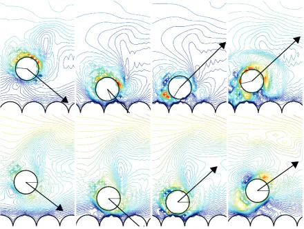
Figure 6.Velocity field (ux(t),uy(t)) resulting from interaction of the particle and the fluid for the rotating (upper row) and non-rotating-particle (lower roe). Sequence of four detailed snapshots illustrates the velocity field around the saltating non-rotating-particle in free motion, before and after the collision for either rotating or non-rotating case. It can be seen that in the vicinity of the rotating particle the flow velocity is larger and fluctuates more intensely due to the greater total velocity on the particle surface than in the non-rotating process.

Among the prospective beneﬁts of the simulation could be possibility to simulate input parameters from wide ranges and examine initial and boundary conditions which may be diﬃcult to prepare experimentally. Thus it could also serve as a guide or help for design of prospective experiments.

References

1. U. Frisch, B. Hasslacher, Y. Pomeau, Phys. Rev. Lett. 56, (1986) 1505-1508
2. G. R. McNamara, G. Zanetti, Phys. Rev Lett.61, 1988 2332-2335
3. S. Succi, The lattice Boltzmann equation for fluid
dy-namics and beyond(Clarendon, Oxford, 2001)
4. J. G. Heywood, R. Rannacher, S. Turek, Int. J. Num. Meth. Fluids22, (1996) 325-352
5. R. Kurose, H. Makino, S. Komori, J. Fluid Eng. Trans ASME123, (2001) 956-958
6. Y. Ni˜no, M. Garcia, Water Resour. Res. 30, (1994) 1915-1924
7. N. Lukerchenko, Z. Ch´ara, P. Vlas´ak, J. Hydraul. Res. 44, (2006) 70-78
8. A. J. C. Ladd, J. Fluid Mech.271, (1994) 311-339 9. C. K. Aidun, Y. Lu, E. J. Ding, J. Fluid. Mech. 373,
(1998) 287-311
10. P. Lallemand, L. S. Luo, J. Comp. Phys.184, (2003) 406-421
11. Q. Zou, X. He, Phys. Fluids9, (1997) 1591
12. M. Junk, Z. Yang, Prog. Comp. Fluid Dyn.8, (2008) 38-48
13. M.P. Allen, D. J. Tildesley,Computer Simulation of
Liquids(Clarendon, Oxford, 1987)
14. J. Latt, B. Chopard, Math. Comp. Sim.72, (2006) 165-168
15. J. Latt,Hydrodynamic limit of lattice Boltzmann
equa-tions(Ph.D. Thesis, Univ. Gen`eve 2007)
16. S. Ansumali, I. V. Karlin, J. Stat. Phys.107, (2002) 291-308
17. S. S. Chikatamarla, S. Ansumali, I. V. Karlin, Phys. Rev. Lett.97, (2006) 010201
18. L. Wang, Z. Guo, Ch. Zheng, Comp. Fluids39, (2010) 1542-1548
19. Z. Yu, L. S. Fan, J. Comp. Phys.228, (2009) 6456-6478