Data-Driven Methods for the
Assessment and Improvement of
Forecasts
Suja M. Aboukhamseen
Department of Statistical Science University College London
Thesis subm itted for the degree of Doctor of Philosophy Faculty of Science, University of London
ProQuest Number: U643637
All rights reserved
INFORMATION TO ALL USERS
The quality of this reproduction is dependent upon the quality of the copy submitted.
In the unlikely event that the author did not send a complete manuscript and there are missing pages, these will be noted. Also, if material had to be removed,
a note will indicate the deletion.
uest.
ProQuest U643637
Published by ProQuest LLC(2016). Copyright of the Dissertation is held by the Author.
All rights reserved.
This work is protected against unauthorized copying under Title 17, United States Code. Microform Edition © ProQuest LLC.
ProQuest LLC
789 East Eisenhower Parkway P.O. Box 1346
A bstract
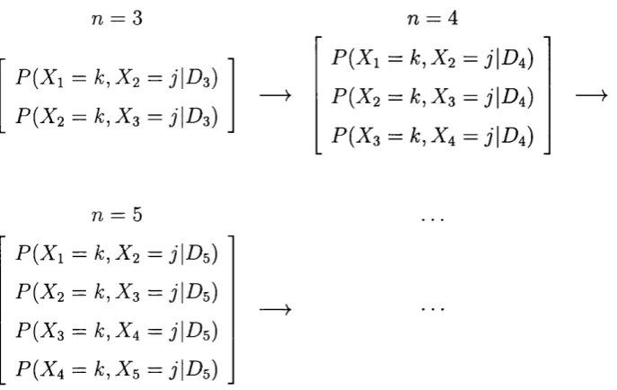
This thesis uses data-driven techniques to analyse and assess both point and probability forecasts within a prequential framework. Point forecasts are assessed using recursive residuals. Examination of the properties of the recursive residual found them to be unique to this residual. Recursive resid uals for the hidden state of HMM are also defined by taking the difference between the one step ahead forecast and the forecast’s filtered update. The quality of forecasts generated from different models can be assessed by com paring the information content in their corresponding residuals. When faced with model misspecification it is shown how this residual can be modelled to correct this misspecification, thereby improving forecasts. It is also shown how the residual content can be used to judge the predictive sufficiency of alternative forecasting methods. Using the theory of probability forecasting, the technique of forecasting assessment by calibration is extended to HMM’s to assess how well the one step ahead forecast is explained by its filtered update. A test statistic to test the empirical calibration of the forecasts is also defined and applied to the real world problem of CpG island detection in Human DNA sequences. The distribution of the test statistic is investigated
using a prequential frame of reference and is found to be N { 0 ,1). Calibration
Acknowledgements
I would like to express my deepest gratitude to my supervisor Prof. A. P. Dawid for his guidance, patience, and time. For the opportunity of being his student, I feel truly privileged.
I would also like to thank my parents, and my brothers and sisters for their unwavering faith, unfaltering tolerance, and continuous encouragement.
To my fellow students and staff at the Department of Statistical Science, and to all the friends th a t I have made all over the UK, I would like to express my sincere thanks for their friendship, encouragement and help. A special thank you to my colleague Kai-Ming Chang who has shared the Ph.D. experience with me.
Contents
A b stra ct i
A ck n ow led gem en ts ii
List o f F igures v i
List o f Tables v iii
1 In tro d u ctio n 1
1.1 Hidden Markov M o d e ls... 2
1.2 Prequential A n a l y s is ... 4
1.3 Probability forecasting and c a l i b r a t io n ... 5
1.4 Outline of T h e s i s ... 8
1.5 Basic C o n c e p ts ... 9
1.5.1 M a rtin g a le s ... 9
1.5.2 Conditional In d e p e n d e n c e ... 11
2 T h e R ecu rsive R esid u al 12 2.1 In tro d u c tio n ... 12
2.2 Recursive R e sid u a ls... 13
2.3 LUS R esid u als... 15
2.5 R e s u lts ... 18
2.6 D iscu ssio n ... 26
3 M o d ellin g R esid u als 27 3.1 In tro d u c tio n ... 27
3.2 Ordinary Least Squares Residual ... 29
3.2.1 The correct model ... 30
3.2.2 Correcting misspecified models ... 32
3.2.3 R e s u lts ... 34
3.3 Recursive r e s id u a ls ... 35
3.3.1 OLS and recursive residual r e la tio n s h ip s ... 35
3.3.2 The correct model ... 36
3.3.3 Modelling recursive resid u als... 38
3.3.4 R e s u lts ... 41
3.4 Residual Analysis in Bayesian M o d els... 41
3.4.1 The predictive d istrib u tio n ... 41
3.4.2 The two stage a p p r o a c h ... 44
3.4.3 C o n f irm a tio n ... 46
3.4.4 Alternative justification ... 47
3.5 D isc u ssio n ... 49
4 H id d en M arkov M od els and R ecu rsive R esid u als 51 4.1 In tro d u c tio n ... 51
4.2 Hidden Markov M o d e ls... 52
4.3 Recursive Residual Applications in H M M s ... 54
4.4 R e s u lts ... 56
4.5 G en eralisatio n ... 58
4.7 D ata Compression ... 63
4.7.1 Compression of l i ... 63
4.7.2 P ro o f... 64
4.8 Sufficiency... 66
4.9 D isc u ssio n ... 68
5 C alib ration for H id d en M arkov M od els 71 5.1 In tro d u c tio n ... 71
5.2 The Calibration Criterion ... 73
5.3 The Calibration Criterion for H M M s ... 74
5.4 A p p licatio n s... 77
5.4.1 Example 1 ... 77
5.4.2 Example 2 a ... 83
5.4.3 Example 2 b ... 84
5.5 D isc u ssio n ... 88
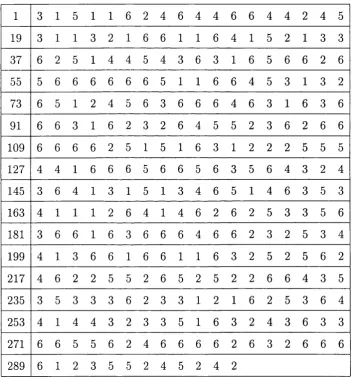
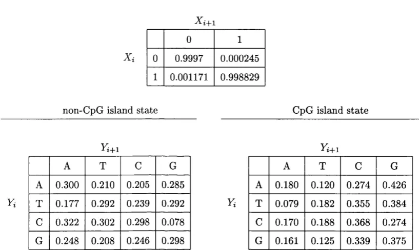
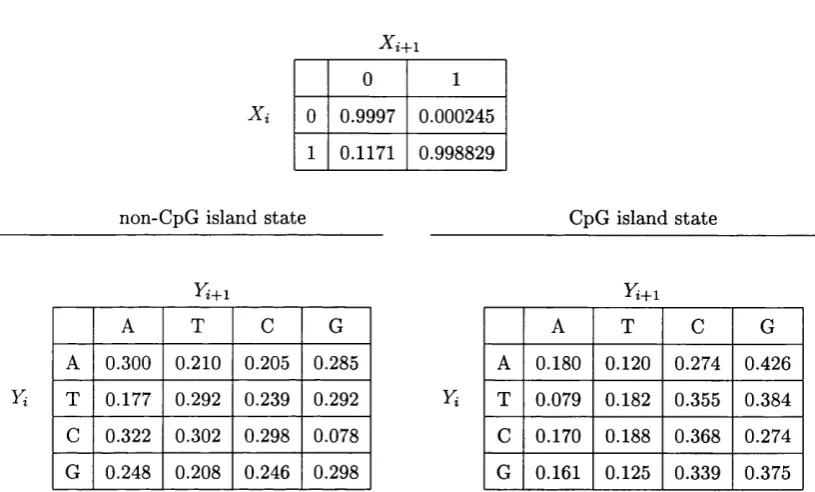
6 C pG Island E xam p le 89 6.1 In tro d u c tio n ... 89
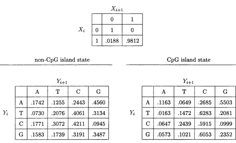
6.2 The Hidden Markov M o d e l... 90
6.3 Assessing C a lib ra tio n ... 93
6.3.1 The test s t a t i s t i c ... 95
6.3.2 Derivation of the test s t a t i s t i c ... 96
6.3.3 Generalisations and re s u lts ... 97
6.4 The Test Statistic D istrib u tio n ... 99
6.4.1 The prequential frame of reference ...100
6.4.2 The production frame of referen ce...105
7 E stim a tio n 109
7.1 In tro d u c tio n ...109
7.2 Baum-Welch estimation ... 110
7.2.1 The EM a l g o r it h m ... 110
7.2.2 The estimation p r o c e d u r e ... 113
7.2.3 R e su lts ...116
7.3 Prequential E s tim a tio n ... 119
7.3.1 Prequential estimation method ...119
7.3.2 Implementation and results ... 124
7.3.3 V a lid a tio n ... 128
7.4 P erfo rm an ce...132
7.5 D isc u ssio n ...136
8 S m o o th ed P red ictio n s 137 8.1 In tro d u c tio n ...137
8.2 The D a t a ...139
8.3 Computing S i... 142
8.4 Calibration ...142
8.5 Cross-V alidation... 144
8.5.1 C a l i b r a t i o n ... 147
8.5.2 Test S t a t i s t i c ...148
8.6 D isc u ssio n ... 155
9 C on clu sion 161
List of Figures
4.1 HMM diagram ... 53
4.2 D A G ... 55
4.3 Hamilton m o d e l... 61
4.4 Reduced Hamilton m o d e l... 61
4.5 HMM before compression ... 67
4.6 HMM after co m p resio n... 67
5.1 HMM diagram ... 74
5.2 Dice D a t a ... 79
5.3 Ex. 1 plot of forecasts ... 80
5.4 Ex. 1 partial plot (1) of f o r e c a s t s ... 81
5.5 Ex. 1 partial plot (2) of f o r e c a s t s ... 82
5.6 Ex. 1 calibration p l o t ... 83
5.7 Ex. 2b plot of fo recasts... 87
5.8 Ex. 2b calibration p l o t ... 87
6.1 HMM diagram for CPG island d a t a ... 90
6.2 Plot of GpG island f o re c a s ts ... 92
6.3 Calibration plot for CpG island e x a m p l e ... 94
6.4 Prequential frame of re fe re n c e ... 102
6.6 Production frame of r e f e r e n c e ... 105
6.7 Normal probability plots (p ro d u ctio n )... 107
7.1 Evolution of ( 7 .9 ) ... 121
7.2 Evolution of a ...124
7.3 Calibration plot using Baum-Welch estimates ...134
7.4 Calibration using Prequential e s tim a te s ... 135
8.1 Simulated state se q u en ce... 141
8.2 Plot of smoothed p red ictio n s...143
8.3 Calibration plot (smoothed p r e d ic tio n ) ... 146
8.4 Cross-validation calibration p l o t ... 150
8.5 Cross-simulation m e th o d ... 152
8.6 Production m e t h o d ... 153
8.7 Normal probability plots (cross-sim ulation)...157
List of Tables
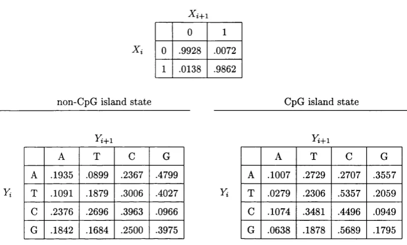
6.1 CpG island m o d e l... 91
6.2 Calibartion for CpG island e x a m p le ... 93
6.3 Test statistic results ... 98
6.4 Prequential simulation r e s u l t s ... 104
7.1 Baum-Welch estimation f o r m u l a s ... 114
7.2 Initial param eter values ... 117
7.3 Baum-Welch param eter e s tim a te s ... 119
7.4 MLE starting values ...126
7.5 Prequential estimates using MLE strating v a lu e s ... 126
7.6 Prequential estimates (second s c e n a rio )... 127
7.7 Converged prequential estimates (scenario 1 ) ...130
7.8 Converged prequential estimates (scenario 2 ) ...130
7.9 Test run starting values ... 131
7.10 Converged estimates for test r u n ... 131
7.11 Calibration results using estimates ...133
8.1 Simulation m o d e l ... 140
8.2 Calibration results (smoothed p r e d ic tio n s ) ... 145
8.3 Cross-validation calibration results ...149
Chapter 1
Introduction
This thesis will address the problems of forecasting improvement when faced with model inadequacy and the problem of forecasting assessment in an information-restricted situation represented by hidden Markov Modelling.
The motivation behind this work draws heavily on the distinction be tween statistical models and the physical reality these models attem pt to represent. A model is proposed in the hope of providing an explanation for a real world problem: a coherent statistical representation based on the mod
eller’s subjective interpretation of the data generating system. Since the true
mechanics of a data source are not known, the only link between the physi cal world and the statistical world used to represent it is the d ata observed. Based on this, the focus of this thesis is on the use of data-driven techniques in statistical analysis as a method of assessing and improving forecasts.
will be judged by the quality of the forecasts they generate at each inter mediate point in time for the next observation, based on analysis of earlier outcomes. In this thesis, both point forecasts and probability forecasts are constructed and analysed within the prequential framework (Dawid, 1984), using the formalisms of probability forecasting (Dawid, 1986).
The prequential approach to data analysis (Dawid, 1984) is customised for the data-driven analysis of real world problems and the sources th a t emit them (Dawid, 1992). Therefore, the prequential approach, being an essen tially d ata analytic approach, is adopted as the general theoretical framework for the concepts developed.
This thesis is dedicated to the development of new empirical methods for the analysis of data and the assessment of forecasts, and the extension of already existing methods of empirical assessment in various applications, hidden Markov models in particular (refer to section 1.1). In the case when point forecasts are made, the data are analysed by defining and using recur sive residuals. In the case of probability forecasts, the field of probability forecasting has developed a rich literature of probability forecasting assess ment techniques, the primary focus of which is calibration (explained in sec tion 1.3). Here, these calibration techniques are extended to applications in hidden Markov models.
1.1
Hidden Markov Models
Researchers in many different fields have found treating a sequence of observations, as part of a causal formation such as the one described above to be very useful. Although these modelling techniques have been in use in various fields of engineering for some time now, interest was rekindled with Rabiner’s 1989 article on HMMs. Since then HMM modelling has been applied in variety of different fields. In econometrics, Hamilton (1988, 1989,
1990, 1993), Harvey (1993), and McCullock and Tsay (1994) use
switching-state space models to model data where the dynamics of an observed time series are considered to change according to a non-observed Markov chain. Hamilton (1989) and Kitagawa (1987) have both developed variations of filtering and smoothing algorithms for this sort of model. HMM modelling has also be applied extensively in the fields of computational biology (Krogh 1994, 1998) and speech and pattern recognition (Jaung and Rabiner,1991). A review of the use of HMMs in protein and DNA sequencing can be found in Biological Sequence Analysis by Durbin et al (1998). Churchill (1992) and Crowley et al (1997) also give examples of other HMM applications in genetics.
viewed as examples of a dynamic Bayesian network.
Throughout the thesis, the term HMM will be used as a general term to encompass all these modelling techniques.
1.2 Prequential Analysis
The prequential approach to statistics (Dawid, 1984, 1996) is characterised by three main features:
1. The formalisation of the procedure involved in making forecasts for the future and assessing these methods on their empirical success at this task.
2. Offering suitable measures of uncertainty for unknown events where uncertainty is expressed in the form of a numerical probability.
3. Considering the sequential nature of the forecasting task.
The basis of this approach to statistics is the “appropriate m anipulation of the d ata currently available so as to produce a specific probability distribution for the next observation” (Dawid, 1985) under the supposition th a t the d a ta arrive in sequence. The prequential method can also accommodate situations which only require a point forecast or a decision problem. At any time z, a probability distribution, P^+i, is formulated expressing uncertainty about the
outcome of the next observation, in the light of the outcomes observed
so far. In the case when a point forecast is needed, this formulation can be applied to solve the problem at hand. The term prequential refers to the combination of probability forecasting with sequential prediction.
estim ation is considered only in its capacity to improve the predictive perfor mance of the prequential forecasts generated. The success of the estim ation task is determined by the quality of the forecasts it helped to produce. The predictive performance is assessed through the comparison of the forecasts with their outcomes.
1.3
Probability forecasting and calibration
The development of probability forecasting as a theoretical discipline came about through the work of meteorologists in their use of probabilistic weather forecasting. The uncertain nature of the weather requires forecasters to quantify their degree of belief about the outcome of rain (Probability of Precipitation) on any given day. Each day a weather forecaster issues a PoP for the next day using all the information available. Come the next day, the outcome of yesterday’s uncertain event is now known. Adding this newly ac quired information to the forecaster’s information base, the forecaster again repeats the task of issuing a PoP for the following day. The demands placed upon weather forecasters in issuing daily PoPs has motivated much of the development of the theory and practice of probability forecasting. A detailed review of probability forecasting is given in Dawid (1983). Of primary inter est here are the contributions made in the development of methods for the empirical assessment and comparison of a sequence of forecasts in the light of the outcomes of the forecast events.
In the prequential framework, the probability forecasts issued are con
structed from what is called a prequential forecasting system. Let a =
(tti, 0 2, . . . ) denote the sequential outcomes of uncertain events A = (Ai, A2,. ..)
where Ai = 1 the event occurs and = 0 if the event does not occur
(i > 1). In light of the observed outcomes at time z, a probability, must be assigned to the outcome of the next event A^+i. Any m ethod of constructing sequential forecasts for every i and = (oi, 0 2, . . . , in this way is called a forecasting system Dawid (1985). A prequential forecasting system is defined by a rule which associates a choice of for every i and with any possible outcome a^) — (ai, 0 2, . . . , Gj) of = ( ^1, ^2, . . . , A^).
Probability forecasts are assessed by determining how successful a fore casting system, F , which constructs the sequence of forecasts, is in explaining the sequence of outcomes. In the case when Ai € {0, 1} is binary, the crite rion chosen to judge probability forecasts is calibration. In the meteorology literature calibration is referred to as validity (Miller, 1962) or reliability (Murphy, 1973). Lichtenstein et al (1982) give a review of the literature on the application of calibration in both meteorology and other fields.
The second task, labelling, refers to the assigning of a numerical value to the common probability in each subsequence. Calibration only addresses a forecasting system ’s labelling ability.
In DeGroot and Fienberg (1982, 1983), sorting is referred to as refinement. They address the issue of inadequate well-calibrated forecasters and show how some well-calibrated forecasters can be deemed superior to others by comparing their refinement.
The forecasting assessment criterion of calibration is formalised in Dawid (1982) with the presentation of a general calibration theorem. Supposing th a t the forecasts arise sequentially from a joint probability distribution P , this criterion requires th at, for an arbitrarily selected test set (where the selection
process is admissible), the difference between the proportion of times in which
an event in question occurs and the average forecast probability for those times tends to zero, as the number of forecasts considered in the test set approaches infinity. Any forecast system F which meets this criterion for the selected test set is said to be completely calibrated, thereby deeming F an empirically valid explanation for the sequence of outcomes. A sequence of forecasts which satisfies this criterion of complete calibration has both perfect calibration and maximum attainable resolution. As such, it can be shown th a t if, by the complete calibration criterion, two forecasting systems, F^
and are considered to be valid explanations for a sequence of outcomes,
a, with corresponding forecast sequences and p^, then pj — pf — > 0 as
i — )■ oo (Dawid, 1985). The calibration criterion satisfies the m eta criteria laid out by Dawid (1985) for the selection of an appropriate criterion for the assessment of the empirical validity of a forecasting system.
1.4
Outline of Thesis
In a situation when point forecasts are made, recursive residuals (Brown et al, 1975) are used as the data-driven apparatus of the forecasting assessment techniques. Hadi and Son (1989) examine some of the distinctive properties of the recursive residual. In Chapter 2, it is shown how the properties of a recursive residual are, in fact, unique to this residual alone, determining its structure.
Although recursive residuals are commonly used as a diagnostic mecha nism (Harvey, 1990), Lumsdaine and Ng (1999) have shown th a t they can also be used to improve the performance of linear models by adding cumu lative functions of recursive residuals to the regression equation. A variation of this concept is explored in Chapter 3 where the recursive residuals of a misspecified linear model are used in the formulation of a new model. Ex am ination of the residuals of the new model show th a t the information lost through misspecification is regained by modelling the residuals in this way which produces the same results as a model th a t has been correctly specified. Chapter 3 also shows how recursive residuals can be defined and applied in Bayesian scenario.
Recursive residual applications are extended to the scope of HMMs in Chapter 4 where the residuals are defined and analysed for the unobserved state of various hidden Markov models. Using these definitions it is possible to show how a sufficient statistic for such models can be constructed and applied.
plications in HMM configurations. Using the real world problem of CpG island detection in human DNA sequences, Chapter 6 illustrates how cali bration can be used in the assessment of forecasts generated from HMMs, and presents a test statistic for testing the empirical validity of such fore casts as set out by the complete calibration criterion. The role of estim ation in improving forecasts is examined in Chapter 7 using the DNA sequence data. A prequential online estimation method for HMMs is given and the calibration of forecasts constructed from param eter values estim ated using both this method and the more common Baum-Welch (Rabiner, 1989) esti m ation algorithm are scrutinised. The calibration criterion is also examined outside the prequential framework in Chapter 8 using smoothed predictions and cross-validation forecast assessment.
1.5
Basic Concepts
Described below are two concepts th a t are used frequently throughout the thesis.
1.5.1 M artingales
Let (Wi, %2, A^3, • • •) be a sequence with finite mean. The sequence is called a m artingale if the conditional expectation of Xi+i given the values
X i , X2, i s equal to
E { X i + i \ X i , X 2t ■ ■, X i ) = X i . (1.1)
A m artingale can also be defined in the following, more general, way. Let A
be a cr-field such th a t A Ç Then it is required th a t Xi be ydj-measurable
for all i, and
In such a case, (%*) is said to be a martingale adapted to the filtration (A). Then (1.1) is recovered when f t is the cr-field generated by ( X i , . . . ,Xi).
Let Si = X i and let Si = Xi — X^_i for all i > 2. Then the constraints (1.1) and (1.2) can be written as
E ( f t+ i|f t, 5 2 , . . . , ft) = 0
and,
E ( f t + i | f t ) = 0 , (2 = 1, 2, . . . ),
and the sequence of variables (5%), for 2 = 2, 3, . . . , is said to form a m artingale difference sequence with respect to (ft).
T h e o re m 1.1 Let the series {Xi) be a martingale difference sequence, so that E { X i ^ i \ X \ , X2, . . . , Xi) — 0 (2 ^ 1), and define f t = X i -I-X2 + • • • TX%. f t Q, (2 > 1), is a predictable sequence of random variables such that Ci <
Ü2 < . . . — >00 and
0 0
Z <0 0 (1.3)
k=l
hold with probability one, then with probability one
c-^Ui 0, (1.4)
and the variables
= (1.5)
converge to zero.
The proof can be found in Feller (1971, pg. 238). The sequence (ft) is a
martingale sequence and E{Y^) is bounded by the series in (1.3). By the M ar
tingale Convergence Theorem, the sequence (ft) converges with probability one and condition (1.3) holds true for each point in the sample space where (ft) converges. From Kronecker’s lemma (Feller, 1971) the convergence of
1.5.2
C onditional Independence
Let y , and Z denote discrete random variables with a joint distribution
P. The conditional distribution of X given Y = y, where y is any possible outcome of Y subject to P { Y = y) ^ 0, is denoted by P { X \ Y = y). Two random variables X and Y are said to be marginally independent, denoted by X IL T , if
p ( x | y = 3/) = f ( X) ,
for all possible values y for Y meaning th a t the probability of X is indepen dent of the outcome of Y . X is said to be conditionally independent of Y
given y , denoted as X A L Y \ Z if, for any possible values y and z for Y and %,
P ( % | y = ? / , Z = z ) = P ( X | Z = z ) .
All the definitions and properties in this section apply to both the discrete and the continuous case, but suppose for simplicity th at %, Y , and Z are discrete random variables assuming any possible values x, y and z respec tively. Let a(a:,z), b{y,z) denote unspecified functions of (x, z) and {y, z)
respectively. Then X A L Y \ Z if and only if any of the following equivalent conditions holds:
1. (a
(b
2. (a
(b
3. (a
(b
(c
P{x\y,z) = P{x\z) if P ( y , z ) > 0
P{x\y, z) has the form a{x, z) if P{y, z) > 0.
P{x ,y\z) = P{x\z)P{y\z) if P{z) > 0
P{x,y\z) has the form a{x, z)b{y, z) if P{z) > 0.
P{x, y, z) = P{x\z)P{y\z)P{z)
P { x , y , z ) = P { x , z ) P { y , z ) / P { z ) if P (z) > 0
Chapter 2
The Recursive Residual
2.1
Introduction
Residuals are the core of the forecasting assessment methods used in this thesis. Essentially, the residual is a linear function of the discrepancy, y —
between an observed value y and its prediction y. Depending on the m ethod of formulation of y, and the linear transform ation o i y — y chosen, any number of different residuals can be produced. This flexibility enables the selection or formulation of residuals with certain desirable properties and characteristics.
The analysis carried out in this thesis is, for the most part, performed w ithin a prequential framework. To remain with the limits of this framework the residual used must also be prequential in nature. The recursive residual (Brown et al, 1975) is one such residual. Described in greater detail in section 2.2, the formulation of the recursive residual is such th a t it provides
a fair and sequential assessment of forecasting performance by using only
d a ta observed prior to the observation of event y in the formulation of y.
(Dawid, 1985).
This chapter examines the various characteristics and properties of recur sive residuals. It is shown how the properties of this transform ation vector, expressed in terms of a residual transformation m atrix, determine its compo nents thereby, proving th at the properties possessed by the recursive residual are unique to this residual.
After the recursive residual is briefly introducted in section 2.2, a broader family of residuals, the Linear Unbiased Scalar (LUS) residuals is described in section 2.3. The formulation of the LUS residuals and their corresponding residual transform ation matrices paves the way for the introduction of the recursive residual transformation matrix. The structure and properties of this m atrix are given in section 2.4, and section 2.5 shows how the properties of the m atrix determine its elements.
2.2
Recursive Residuals
Consider the simple linear regression model
Y = X6» 4- e, (2.1)
where Y is a n x 1 vector of observations on the dependent variable, X is a n X p m atrix of rank p consisting of observations corresponding to the p
independent variables, ^ is a p x 1 vector of unknown parameters, and e is the n X 1 vector of unobserved disturbance terms with expectation zero and
th a t disturbance term is (0, cr^), the recursive residual is defined as
W, = , ~ , (2.2)
y i + X i( X T ,X ,_ i) -'x T
where yi is the observation of Y and §i_i = X^^Y%_i is the
least squares estimate of#. It is im portant to note here th a t #j_i is evaluated
using only the data observed up to and including time i —1. The estim ate for 6
specified in this way gives the residual a prequential quality. The predictions,
yi = X{9i-i, generated using this formulation of 6 are also prequential which, in turn, makes the recursive residual a prequential diagnostic mechanism.
Brown, Durbin, and Evans (1975) introduced the recursive residual for the standard linear regression model as an alternative to the ordinary least squares residual which will be discussed in greater detail in Chapter 3. In analytical terms, the recursive residual is merely the prediction error resulting
from the difference of yi from its prequential prediction yi = Consider:
var [yi - yi] = var (x^# + Ci) - ^x^ (x f_ iX i_ i) ^ X ^ ^ Y ^ .i^
= var [ci] + Xi (x f_ iX i_ i) ^ Xj_^var [X^_i# + X^_i ( x f_ iX i_ i) ^ x
= + Xi (x f_ iX i_ i) ^ xfo-^
= cr^ (^1 + Xi (xf_iXi_i) ^
xf^ ,2.3
LUS Residuals
The recursive residual belongs to a family of residual known as Linear Unbiased with Scalar Covariance M atrix (LUS) residuals. Introduced by Theil (1965, 1968, 1971), residuals within this family are characterised by a residual vec tor th a t is linear and unbiased. In addition, the residual vector is subject to the constraint th at its covariance m atrix be scalar, i.e. it can be w ritten
in the form Using the above, the properties of residual transform ation
m atrix, C of a LUS residual vector are:
1. The residual transformation m atrix C is an {n — p) x n m atrix not involving Y . The rows of C are characteristic vectors of the m atrix (I — H ) corresponding to unit roots. The rows of C all have unit length and are also pairwise orthogonal.
2. C X = 0, so th a t the expectation of the residual vector,
E[ CY] = E [ C { X e + e)]
= 0,
is equal to the expectation of the disturbance term ensuring th a t the vector is unbiased.
3. C ^ C = (I - H ), where H = X ( x ^ x ) ” ^ X ’’.
4. C C ^ = I, where I is the identity m atrix so th at
n ar [CY] = n ar [C (X0 + e)]
= var [Ce]
= er^CC^
= (7^1
Theil’s notion of an unbiased residual vector is explained below. Con sider the standard linear model in (2.1). The least squares residual vector is expressed as
e — Y„_p — Xn_p0 (2.3)
= C Y ,
where C is the residual transformation m atrix not involving Y , e is the
{n — p) X 1 residual vector, Y „-p and Xn_p are the (n — p ) x l and {n — p ) x p
submatrices containing the last (n — p) elements of Y and X respectively, and 9 is the least squares estimate of 9. Recall th at the n x 1 vector of disturbances, e is unobserved. Expressed as
e = Y - X6>,
it is easy to see th a t the residual vector offers itself as a natural approximation for at most n — p components of e. Consequently, if the residual vector is regarded as an estimate of e, then it is unbiased if E[e] = E[e] which, in this case, is equal to zero.
The conditions of unbiasedness and scalar covariance imposed on C imply th at only n — p residuals can be found. Such conditions require th a t p of the disturbance terms be discarded. From C X = 0 it is possible to see th a t the n columns of C are subject to p linear dependencies. As such p of the disturbance terms can be discarded without any loss of information.
2.4
Recursive Residual Transformation M atrix
Consider the unstandardised recursive residual,
i — Vi (2.4)
i = p + 1, . . . , n. The recursive residual vector, being a member of the LUS family of residuals (Hadi and Son, 1989), can be expressed in terms of a residual transform ation matrix. Let B denote the (n — p) x n recursive resid ual transform ation m atrix for the unstandardised recursive residual vector r satisfying
r = B Y .
Then, B is of the form
-X p+2 {Xp+l^p+l)
1 0 . .
1 0
1 0
Let bij denote the element of B on row i and column j where i = (n —p). n and j = 1 , . . . , n. The transformation m atrix B has a lower triangular structure with all the i < j elements equal to zero and bij = 1 for all i = j elements of B. The remaining i > j elements are defined separately for each
of the i rows of B by the 1 x {n - i) vector — X^_^.
The recursive residual transformation m atrix possessess all the properties of a LUS transform ation m atrix discussed in section 2.3. It is, however, mentioned th a t B is not the standardised recursive residual transform ation m atrix. The rows of B, although not normalised, remain pairwise orthogonal. Due to this, B B ^ is a diagonal dispersion m atrix with diagonal element
equal to the square of the standardising constant of the row of B. In order
residual transform ation m atrix in its unstandardised form has the advantage of simplifying the algebraic manoeuvres in the next section.
2.5
Results
Let B denote the standardised version of the recursive residual transfor m ation m atrix, B, specified in the previous section. Then, in addition to possessing all the properties of a LUS residual transform ation m atrix listed in section 2.3, B also has the following two properties:
1. B is (n — p) X n m atrix
2. bij = 0 for z < j
which are specific to the matrix.
T h e o re m 2 . 1 Given the above properties of the recursive residual trans
formation matrix, the formulation of the recursive residual transformation matrix is unique.
P ro o f. Except for i > j elements, the above properties of B define all the characteristics and elements of B. The remaining i > j elements can be solved for using a system of equations provided by B X = 0 and B B ^ = I.
Let Bij denote a j-length row vector containing the first j elements of the i^^
row of B. is an arbitrary row in B. The value of is determined
by a set of p linearly independent equations from = 0 or equivalently
from Bi+ ij+iXi^i = 0 since Bi+ij+i contains the first z -fl elements of Bi+i^n and the remaining elements are equal to zero. The remaining i —p equations come from Bi+i.i+i [A] = 0, where A =
known.
Assume th at rank{Xp) = p, then it follows th a t the rank of X^+i, where (ï + 1) > p, is also p. Assume, also, th a t the diagonal elements of B are
positive. Then [A X^+i] = 0 gives a homogenous set of i equations
in i unknowns. For the solution to be unique it is sufficient th a t A be orthogonal to X%+i. A is nothing more then a subset of the first i rows of B , where only some of the trailing zeros have been left out. W ith this in mind, the orthogonality of A and Xj+i follows from B X = 0.
The concept outlined above will now be implemented to derive the exact formulation of the recursive residual transformation vector. For simplification the m atrix B is replaced by B. The first three rows of B will be solved for initially to establish the recursive structure of the evaluation scheme. Induction will then be used to generalise the results for the remaining rows of B.
Let Bj denote the row of B and let A j denote a j-length row vector
containing the first j elements of the row of B. The m atrix X is partitioned
in the following way
Xp Xp+i Xp-f-2 X =
S o lv in g for Bp+i Expressed in terms of A + Lp? ®p+i has the form
Bp+i (^p+l,p; f 5 bj • • • 1 b)
Multiplying Bp+i by X yields the first row of B X . Since B X = 0, the result is a 1 X p vector of zeros:
so th at
Bp+i,p^p — ~Xp+i- (2.6)
The 1 X p vector in (2.6) is a system of p equations in p unknowns
providing a unique solution for the unknown elements in Bp^i^p since Xp is a (p X p) m atrix of full rank. Using this system of equations
solving for Bp+i^p is trivial:
Bp+i^p —Xp-i-i (Xp)
= - X p + i ( x J X p ) " 'x J '
which is exactly as desired.
S o lv in g for Bp+2 The same procedure used to solve for Bp+i is followed here to solve for Bp+2- First, Bp+2 is multiplied by X which (from
Bp+2^ = 0) yields:
Bp-\-2,p^p T ^p+2,p+iXp-f 1 Xp^2? (2.7)
a system of p equations in p + 1 unknowns. It is, however, possible to express one of the unknown component 6p+2,p+i in terms of Bp^2,p
using the m atrix B B ^ B B ^ is a diagonal m atrix which means th a t any row of B multiplied by any other row of B, other than itself, is equal to zero. Multiplying Bp+2 by B ^ ^ gives
Bp+2Bp+2 = Bp^2,pBp^ip + 6p+2,p+i = 0
which can be rearranged to give
^p+2,p+i = ~^p+‘2,pBp^i^p. (2.8)
Let Cp+i = - B j+ i p, so th at
and note th a t X ^Cp+i =
xp+i ( X ^ X , ) ' X j
T
■p+1 = X % ( x % ) ' ' x
-— ^p+1
-Although it is not yet apparent, the specification of Cp+i and future Ci’s (z = p + 2, . . . , n — 1) plays an im portant role in clarifying the recursive nature of the algebra used in this proof.
Expressed in terms of Bp+2,p, ^p+2,p+i can be substituted for in equa tion (2.7) giving a linear system of p equations in p unknowns:
-^p+2,p^p "b 6p+2,p+l^p+l — ~Xp+2 -^p+2,pXp + B p ^ 2 , p ^ p + l ^ p + l ^p+2
B p + 2 ,p (Xp 4- Cp+iXp+i) = — Xp+2 It is now possible to solve for Bp+2,p:
-^p+2,p — ^p+2 (Xp 4- (7p-)-iXp^i) (2.9)
= — Xp+2 (Xp + Cp+iXp+i) ^ (X p) X.p
= —Xp+2 (XpXp + XpCp+iXp+i) Xp
= —Xp+2 (XpXp 4- Xp_^^Xp_|_i^ Xp
= -X p+2 (Xp+jXp+i) Xp.
Using the value of Bp+2,p derived in equation (2.10), 6p+2,p+i can be evaluated:
^p+2,p+l — -Sp+2,pC*p+l (2 1 9 )
= -X p+2 (x J^ jX p + i) XpCp+1
Xp+l-Together, Bp+2,p and 6^+2,p+i niake up the vector Bp+2,p+i = [Bp+2,p bp+2,p+i],
the unknown components of the row Bp+i. Substituting Bp^2,p and
bp+2,p+i with the values obtained in (2.1 0) and (2.1 1) gives the com plete composition of Bp+2,p+i,
B p + 2 , p + l — [ B p + 2 , p b p j^ 2 , p + l]
— Xp+2 (Xp+iXp+i ) " x
-= "Xp+2 IXp+iXp+1^ " [X?
— "Xp+2 IXp+iXp+i)
X Xp+2
u
- 1 (Xp_|_iXp+i I XTp + 1
S o lv in g fo r Bp+g First, p linear equations are obtained from Bp+gX = 0,
- S p + 3 , p X p + 6 p + 3 , p + i X p + i + 6 p + 3 ^ p + 2 X p + 2 = — X p + 3 . ( 2 . 1 1 )
The computations become more complicated as the difference between
p and i, i = {p-\-l), . . . , n, becomes larger. As in the case of Bp+2, the scalars 6p+3,p+i and 6p+3^p+2 are expressed in terms of Bp+3,p using the composition of the m atrix B B ^. The table below shows the expressions obtained for 6p+3^p+i and 6p+3 p+2
-Rows Multiplied Expression Obtained
Bp+3B^2 = 0
Rp+3,pRj+i p + &p+3,p+i = 0
bp+3,p +i = —Rp+3,pB^j p
— Bp+3 pCp+i
Bp+3Bp+2 = 0
Bp+s,pBp_^2,p + ^p+3,p+l^p+2,p+l + &p+3,p+2 = 0 ^p+3,p+2 = ~^P+3^p+2,p ~ bp + 3 ,p + lb p + 2 ,p + l
= - B p + 3 B p ^ 2 , p ~ ^P+3,p^J+l,p^p+2,p+l
Where Cp+2 — (^^p+2,p Cp+i^p+2,p+i^ XpCp+2 — ^p+2
-XpCp+2 = ~ ^ p [Bp_^_2^p - Cp+ibp^2,p+i)
= Xp ^Xp ^Xp_)_jXp+i^ Xp_|_2 + Cp+iXp^i ^Xp_|_]^Xp+i^
= XpXp ^Xp_)_2Xp+i^ Xp_,_2 + Xp_|_iXp+i ^Xp_|_jXp+i^ x^
= (x ^ X p + x^+iXp+i) (x^+iX p+i) x^+2
= ( x ^ + ,X p + i) ( x ^ ^ ,X p + i) - 'x^+2 - X^
— ^P+2
Using the above results, it is now possible to solve the system of equa tions in (2.11). By first substituting for the values of 6p+3,p+i and 6p+3^p+2 in equation (2.1 1) so that
-^p+3,pXp + Bp_|_3 p(vp_|_iXp_|_i -j- .Bp_|_3 pCp_|_2Xp_|_2 Xp_|_3
B p + 3 ,p (Xp 4- Cp+iXp+i -h Cp+2Xp+2) = —Xp+3,
Bp+3,p can be derived:
Bp+3,p = —Xp+3 (Xp 4- Cp+iXp+i -f- Cp+2Xp+2)
= — X p + 3 (Xp 4- C p + i X p + 1 C p + 2 X p + 2 ) ^ ( x j ) Xp
= —Xp+3 (XpXp 4- Xp Cp+iXp+1 -I- Xp Cp+2Xp+2) Xp
= - X p + 3 (Xp Xp 4- X ^ i X p + i 4- xJ^2^p+2) Xp
— — X p + 3 (Xp+2Xp+2Xp+2^ Xp .
Substituting the above expression for 5 p+3,p in 6p+3,p+i and 6p+3,p+2 gives their values where
bp+3,p+l — -^p+3,pC^p+l
= -Xp+3 (Xp_^2Xp+2) Xp Cp+I
and
^p+3,p+2 — -Sp+3,pC*p+2
— -Xp+3 (X.p_^2^P+2) X jC p+2
= -Xp+3 (X ^gX p+2) ^p+rT 2
-Now th at all the unknown elements have been determined, and the vector Bp+3^p+2 can now be specified as
-^p+3,p+2 — [-^p+3,p ^p+3,p+l ^p+3,p+2]
/ ——rp \ 1 fp p
— —Xp+3 (^Xp+2Xp+2j I^Xp Xp+^ Xp+2
— —Xp+3 ( ^ J +2^P+2) ^ p+2
In d u c tio n To ensure th at the recursions displayed in the solution of the first three rows of B hold throughout, a proof by induction is used to generalise the results for any î + 1 row of B. It is assumed th a t the results obtained hold for row % of B, so th at
Bi = - X i ( x f _ i X i _ i ) ''x f _ i ,
1 1,
where Q _ i = — p+Cp+i6i_i^p+i+C'p+26i_i^p+2+ • * •, T Q -2^%-i,%-2, and X j C i - i =
The above equations are now used to solve for the B^+i. From B X = 0
Bi+i^pXp + 6^++p+iXp+i + • • • + 6j+i^iXj = —Xj+i (2.1 2)
Rows M ultiplied Expression O btained ^z+i,p+i — Bi^i^pCp-\-i Bi+iBp+2 ^i+l,p+2 Bj_|_i^pC7p_|_2
B i+ iB f_i — Bi^i^pCi—i
Bî+iB^ bi+l,i Bi^i^pCi Ci in the above table is given by the following formula
Ci = —Bjp + Cp+ibi^p+i + • • • + Ci-ibi^i-i,
and to simplify the computations X jC j is evaluated and found to be equal to x f .
At this point it is now possible to compute Bi+i^p. The scalar quantities,
bi+i,p+i, . •., are substituted for in (2.1 2) which gives
(Xp + Cp+iXp+i + • • • + CiXi)
= —Xi+i (Xp + Cp+iXp_|_i + • • • + CfXi) ^ X^
= -X i+i (X^Xp + xJ+iXp+i + + x f x i ) X j
= - X i + i ( x f X i ) " ‘ x J
The scalar quantities, ft^+i^p+i, . . . , bi^i^i, can now be evaluated:
bi+i,p+i Bi^i^pCp^i
= - x ,+ i ( x J 'X i )
-T
“P
- 1
bi+i,p+2 — “ Xj+i ^X fX j) X ‘‘p+l
T
■p+2
bi+i^i = - X i+ 1 ( x f X i) x [
This concludes the proof: the properties of the recursive residual trans formation m atrix determine its components, making these components unique to these properties.
2.6
Discussion
Chapter 3
Modelling Residuals
3.1
Introduction
This chapter explores methods of modelling residuals to correct model mis- specification. Before the topic is examined in detail the purpose of model specification must first be clarified. The process th at generates the d ata is not known. It is not the purpose of model specification to attem pt to discover or even describe the generation process. The purpose of the model specified is merely to extract the main features of the data so as to provide reliable predictions.
Analysing residuals after designating a model which generates these pre dictions provides an accurate indication of the goodness of fit. Any failure the model might have in detecting variation in the d ata is embodied in the residuals. If the model is adequate it follows th a t the residuals will exhibit no apparent pattern, making them appear approximately random e.g. the sum of the residuals is approximately equal to zero (Harvey, 1990).
mately random residuals is given a more precise interpretation using a prob ability integral transformation. Let Ri be the residual for the observation at tim e i, and let Fi denote the conditional distribution function of Ri given
past observations under the model M, “then Ü = (Ui,U2t ■. ,Un) where
Ui = Fi{Ri) should be independent uniform [0,1]” if data arise from M.
Different tests can be used to assess the uniformity and independence of U.
If the model does not account for a predominant characteristic of the data, then this deficiency on the model’s part seeps through and embodies itself in the residuals. This predominant characteristic is now a systematic component of the residual, and, because of this, the residuals no longer fall into the random category (Harvey, 1990). In such a situation, the analysis is reassessed and a new model is specified using the insight gained from the residuals.
Once the residuals have detected model misspecification, the action taken need not involve the determination of an entirely new model. Dawid (1992) suggests th a t the residuals themselves be massaged into providing a better fit to the data. This entails looking at the residuals as observations of a new response variable and modelling it accordingly. By modelling the residuals obtained from a misspecified model it is possible to bring the lost information back into the analysis.
The correction of model specification through the modelling of residuals is the prim ary focus of this chapter. For a standard linear regression model, it will be shown how the residuals of a misspecified model are derived and mod elled producing what will be termed the residual model. This residual model is also analysed and the residuals for this model, the secondary residuals,
are the same, proving th at such a modelling strategy can be used to correct misspecification and produce results identical to a correctly specified model.
The method of modelling residuals to correct model misspecification is applied using three different residuals. Section 3.2 looks at a simple linear regression model and how ordinary least square residuals can be used to correct an inadequate model. The resulting residual of the residual model is found to be the same as th a t of the correctly specified model. The same m ethod is applied in Section 3.3 to recursive residuals which have a slightly more complex structure. Section 3.4 explores how residuals can be defined and used in a Bayesian framework.
3.2
Ordinary Least Squares Residual
For the linear model, one of the more commonly used residuals is the O r dinary Least Squares (OLS) residual. It is easily computed and with it the modeller can determine what im portant factors have been overlooked. The model under consideration is of the form
Y - X 6> + e, (3.1)
e ~ Y"(0, cr^I), where Y is the n x 1 vector of observations on the dependent variable, X is the n x p m atrix of observations corresponding to the p inde pendent variables, 0 is a p x 1 vector of param eters and e is a n x 1 vector of error terms. Using
ê = (X ^X )“ ‘x ^ Y (3.2)
as the least squares estim ator for 0, the predicted value for Y is X0 and the OLS residual vector for this model is
= Y - x ê (3.3)
= ( I - H ) Y
where H = X(X"^X) ^X'^ and (I — H )X = 0. If the model is correctly specified, then the OLS residual reduces to
R = (I - H)e
showing th a t this residual is a linear combination of the true disturbance term, e, with mean zero and variance cr^(I — H ). Under standard regularity conditions, R will also asymptotically converge in distribution to the true disturbance when n is large in comparison to p.
Despite its optimality, the OLS residual is inappropriate for testing the validity of the assumptions made about the disturbance term of a linear model. This assumption states th at the disturbances are independent with
mean zero and variance a^l. In order to check this assumption, it is necessary
for the residuals to mirror the properties of the disturbances (Harvey, 1990). Since the OLS residuals are both correlated and heteroscedastic, they are generally not viewed as a valid diagnostic for testing purposes (Harvey, 1993).
3.2.1
The correct m odel
Assume th a t the correctly specified model is of the form
Y = X 6 T T e, (3.4)
where Z is n x q m atrix of observations on q independent variables, (/> is a
under the correct model in (3.4). By writing model (3.4) in m atrix notation,
Y =
it is possible to obtain a system of two equations with two unknowns: r 1 ' O c '
X z
4>
x ^ x x ^ z - 1
' x - ' O c ’
Y =
z ^ x z ^ z z^ 4>
X ^ Y Z'^Y
X ^ Y Z^Y
X ^ X X ^Z Z^X Z^Z
X ^ X d c + X ^ Z ^
z ^ x ê c +
de 4>
(3.5)
(3.6) from which the estimates of 6 and can be derived:
êc = ( X ^ X ) “ ^ ( X ^ Y - X ^ Z .ÿ )
0 = (Z^Z - Z^HZ)"‘ (Z^ - Z^h) Y
= ( Z ^ ( I - H ) Z ) “' (z^ ( I - H )y ) .
Substituting (3.6) in (3.5) gives the expanded form of 9c,
§C = ( x ^ x ) ' ' ( x ^ Y - X ^ z ( z ^ ( I - H ) z ) “ ^Z'^(I - H ) y ) . (3.7)
W ith the prediction for Y , Ÿ , equal to + Z(J, the residual for this model is
R(7 — Y — — 'ZiO.
= Y - X 0 - Z 0 + HZ<^,
where 9 is given in equation (3.2) since from (3.5),
êc = ê - ( x ^ x ) " ‘ x ^ z0,
and so
X § o = X 0 - HZ0.
3.2.2
Correcting m isspecified m odels
Assume th a t the correctly specified model is of the form given in equa tion (3.4). The model under consideration, however, is model (3.1). The misspecification takes the form of an om itted variable. The OLS residual in this case is
R i = ( I - H ) ( X 6» + Z(/)-t-e).
Because, in this particular situation, the model is deficient the residual does not have the proper structure of an OLS residual. It is no longer a linear combination of ju st the disturbances, it is also a linear combination of the om itted variable Z and param eter </>:
R i = (I - H)Z(/> + ( I - H)e. (3.9)
The model in Equation (3.9) will be referred to as the residual model. Since R i clearly has a linear regression structure, finding an adequate fit for Y can continue by regressing R i on the om itted variable Z.
It is worth noting th a t both Z and e have been transformed. The distri bution of the error term is now N { 0 ,a ‘^{l — H )). Later, it will be seen th a t this transform ation compensates for the information not accounted for in the original fit. In the mean time, generalised least squares is used to find an estim ate for (f).
First the following definitions are needed. Using a Q R decomposition (Schott, 1997),
Q X = 0
th a t from the orthogonality of Q, Q ^Q = Q Q ^ = In and th a t Q iQ ^ = Ip, Q2Q ^ = I(n-p), and Q iQ ^ = 0. From the above definitions, the following relation is obtained
X =
= Q^R* + Q^O
= Q^R*,
and the projection m atrix H can be expressed as
H = X ( X ^ X ) " 'X ^
= Q T R .R :' ( R p '^ R l Q i
= Q fQ i
Similarly, the projection m atrix for the orthogonal complement of the vector space of X , (I — H) can be expressed as I — Q fQ i = Q2Q2 (since Q ^Q =
Q f Q i + Q ^ Q2) and the following relation is obtained
( I - H ) = Q ^ Q2 Q2( I - H ) Q i ’ = Q2Q I’Q2Q2 Q2( I - H ) Q J = I.
Premultipling both sides of the residual model by Q2 gives
Q
2R
1= Q2(I —
H)Z(^ + Q2(I —
H)e,
a transformed version of the residual where the covariance structure of the vector of disturbances is constant,
war-[Q2(I - H)£] = Q z p - H)war [e] (I - H j Q j = £t2Q2( I - H ) Q ^
The least squares estimate derived from regressing Q2-R1 on Q2(I — H )Z is the generalised least squares estimate for (f):
4> = ( z ’’( I - H f Q ^ Q 2( I - H ) z ) " ' z ^ ( I - H f Q j ’Q2( I - H ) Y = (Z ^ (I - H f (I - H )(I - H ) Z ) “ ^Z^(I - H )^ (I - H )(I - H )Y
= (Z ’’( I - H ) Z ) “ 'Z ^ ( I - H ) Y
For this particular model, using generalised least squares estim ation produces an estim ate for th at is equivalent to the least squares estim ate derived by regressing R i on (I — H)Z:
ÿ = ( z ^ ( I - H ) ^ ( I - H ) z ) ' ^ Z ^ { I - H y ( I - H ) Y
= ( Z ^ ( I - H ) Z ) “ ^ Z ^ ( I - H ) Y , (3.10)
assuming (incorrectly) th at the the errors, (I — H)e, are independent and identically distributed. Using this estimate to derive the residual for the latter stage regression yields
R2 = R i — (I — H)Z(^
= Y - X g - ( I - H ) Z ^
= Y — X 0 — Z( ^ T H Z 0 . ( 3 . 1 1 )
3.2.3
R esults
The estim ate for (/> in (3.10) derived for the residual is identical to th a t derived from modelling the correct model in (3.4). The same, however, is not true for 9. The misspecified model in (3.1) and the correct model in (3.4) give two different estimates for 6. The estimate for the correct model, §c^ uses information on both X and Z. The information about Z comes into §c in
In the misspecified model, however, the analysis, for some reason or an other, has not taken Z into consideration. Z only comes into the analysis when the residuals for misspecified model pick up on Z as systematic compo nent in the residual composition. When the residual model is specified, the residuals are regressed on a linear combination of Z, specifically (I — H ) Z. This transform ation adds a new term, H Z, to the regression which compen sates for the information lost in the misspecification of the model. In the misspecified model, H Z 0 is precisely the term missing from 6. The incor poration of H Z in the residual model gives R2 in equation (3.11) the same composition as R c and the final residuals in both cases are the same.
3 .3
Recursive residuals
Recursive residuals are introduced in detail in Chapter 2. This section uses the definitions and properties defined in Chapter 2 to reproduce the results in Section 3.2.
As in Section 3.2, the correct model is of the form
Y = -j- Z(/> -l- 6.
The misspecification begins by modelling Y = -f e and the analysis then
picks up on the missing component by modelling the residual of the deficient model.
3.3.1 OLS and recursive residual relationships
Let the m atrix B be the recursive residual transform ation m atrix defined in C hapter 2 so th a t B Y is the recursive residual vector. The row of B is
where is the 1 x p vector containing the values of the p independent variables of X at time i, and X%_i is the (i — 1) x p m atrix containing the first (i — 1) rows of the m atrix X. Let hi be the standardisation constant:
/i,=
The properties of B can be used to relate the OLS residual vector to its recursive residual counterpart. The OLS residual vector for Y = X0 + e
is R i = (I — H )Y . Using the properties B ^ B = (I — H ), B X = 0 and B B ^ = I (Theil, 1975), the recursive residual vector, Hi r r^ for the above model can be derived by multiplying the recursive residual transform ation vector by the OLS residual vector,
B Y = B B ^ B Y
= B ( I - H ) Y
= B R i
= RlER. (3.13)
3.3.2
The correct m odel
Specifying the recursive residual vector for the correct model first requires the specification of the estimates for the parameters 6, and (j). Let Z^, B^, and Y i be the first i rows of the Z, B, and Y matrices respectively and let H i be defined as Hf = X i(X fX i)” ^ X f. By definition, the recursive residual requires th a t the estimates used in the prediction of p%, the observation Y , contain only information available time i — 1:
êi_i = ( x f _ iX ._ i) “ ‘ (x f_ iY ._ i - Xf_iZi_i (z f_ i(I - H i_ i)Z i_ i)" ‘
= ( x f _ iX ,_ i) " 'x f _ iY i_ i ( x f _ iX i_ i) “ 'x f _ iZ i_ i (Z f_ i(l
-1 ,
for Z = (5 + 1 n, s = max{p, q}. The recursive residual at time i is
— (Vi — Xi§i-i — '^icRR —
9 i
Vi ~ diY j_i — — fjYi_]
9i
~ iUi ~ (di + + fj) Y i_i)
9 i
1 r
— — (dj + 6i + fi) 1
Ui L
(3.14)
where
(3.15) d, = X i(X f_ iX i_ i)“ Xf_i
e, = Xi (x f_ iX ._ i)“'xf_iZ i_i (z f_ i(I -H i_ i)Z i_ i)'' Z^,^-Hi_i%3.16)
f, = z. (Z f_ i(l - H ,_ i)Z i_ i)" ' Zf_,(I - (3.17)
and Qi is the standardisation constant,
Si = (1 + Xi ( x f _ i X i _ i ) ^ x f
+Xi ( x f _ ,X i_ ,) “ ' X f_,Zi_i (Zf_i (I - H i.i) Z i . i ) " ' Zf_i (I - H i_ 0
X i_i ( x f _ i X , , i ) " ' x f + Zi (zfLi (I - H i.i) Z i_ i) " ' z f ) ' . (3.18)
Expressing the results in terms of a recursive residual transform ation m atrix can be done by specifying HcRR as (n — s)-length vector of the Ticrr residuals and the {n — s) x n m atrix C such th at
c is the recursive residual transformation m atrix where the row of C is
1 Ci = —
9i — (dj + + fi) 1 0 (3.19)
3.3.3
M odelling recursive residuals
From equation (3.13) the following regression model is derived:
^ iR R = b y
= B (X.0 + Z(f) + e)
= B Z 0 + Be (3.20)
Unlike the OLS residual model in (3.9), the disturbance term in model (3.20) has a constant variance since B B ^ = I.
To obtain the recursive residuals for model (3.20) the estim ate of (f) at any arbitrary point in time must contain only information available at th a t time. Therefore, a prediction made for z/j+i will use only the information available at time i. The estimate for cj) derived by regressing 'R.îrr on B Z using only the information upto time i is then
* = { z j B j B i Z i Y " Z j B j B i Y i
= { z J { I - H i ) Z i y ' z J { l - H i ) Y . .
Because the estimate for is different for each i = q , . . . , n — 1, the m atrix notation of the secondary recursive residual for the model in (3.20) has a complicated structure.
of the row of B and the vector of length i as
M,: —
where again i = s 1 , .. . ,n. The recursive residual at time i is
= — ( f ' i l R R —
9i ^ '
= ^ (biY i - biZ iM ,Y i)
9i
= — (b* — biZjM i) Yj
9i (3.21)
where gi is the standardisation constant given in equation (3.18). To simplify, equation (3.21) is expressed in terms of the expressions d%, e^, and defined in equations (3.16), (3.17), (3.17) respectively:
hi 'f'i2R R — —
9i h. 9ihi
1
0
+% 0— (df + + fj) 1
— ~ iVi ~ (dz + Gj + f j Y i_ i),
9i (3.22)
where b* = ^ — d i 1 and biZiM i = ^
To present the recursive residuals in terms of a recursive residual trans formation m atrix the following matrices are used: let B be a block diagonal
m atrix with b% denoting the nonzero components of the row of the m atrix
B. The m atrix has the following structure
0 0 0
0 0 bp+1 0
and likewise the matrices Z, M , Y , and the m atrix of recursive residuals,
^ 2RR are defined as
0 0 0 0 0 . . . Q
z = 0 0 Zg+1 0 , M = 0 0 Mç+1 0
0 0 Zn 0 0
0 0 0
Ÿ = 0 0 Ys+1 0
0 0 Yn
where s = m ax{q,p}. W ith m atrix $ = M Y , a diagonal m atrix with as
the diagonal component, the recursive residual m atrix can be w ritten as
^2RR — B Y — B Z $
= (b - z m) y .
Such a formulation produces the recursive residual m atrix, R2izi^, as a diag onal m atrix
0 0 • • • 0
^2RR — 0 0 1^{s+l )2R R 0
0 0 • • ' T n 2 R R
where U2RR, i = (s + 1 ) , . . . , n , is given in equation (3.21). Multiplying ^2RR by a n X 1 unit vector will produce H2rr^ the n x 1 vector of recursive