Volume 3, No. 5, Sept-Oct 2012
International Journal of Advanced Research in Computer Science
REVIEW ARTICLE
Available Online at www.ijarcs.info
ISSN No. 0976-5697
Generic Models for Evaluating Multicast Protocols in Hierarchical Networks
Jackson Akpojaro* Department of Computer Science
Western Delta University Oghara Delta State, Nigeria
Ugochukwu Onwudebelu
Department of Mathematics and Computer Science Federal University, Ndufu,
Abakiliki, Ebonyi State, Nigeria [email protected]
Abstract: In this paper we derive analytic models for evaluating the performance of multicast protocols in hierarchical networks. Specifically, we investigate the properties and costs of setting up and maintaining a multicast distribution tree by different variants of protocol independent multicast (PIM) in two scenarios; where the data source is outside the networks and secondly, where the data source is part of the networks. We derive our models on the assumptions that the networks are symmetrical and nodes responses are not delayed and the maximum amount of merging possibly takes place. In practice, this means that all round-trip times need to be less than the inter-packet arrival times. The symmetry of the networks enables us to assign equal value to both down and up links and then use the number of links traversed by control message packets to compute the performance of the PIM variants. The results of our numerical investigation confirm that in most mean group sizes the PIM-sparse mode (PIM-SM) is more cost-effective than the PIM-dense mode with flood and prune mechanism (PIM-DMFP).
Keywords: Cost-effective, control message, distribution tree, round-trip time, inter-packet arrival.
I. INTRODUCTION
In spite of the technical difficulty in its deployment, Internet Protocol (IP) multicast remains more superior and cost-effective in group communication than Application Layer Multicast (ALM) protocols [9]. This initial difficulty leads to constant stream of published literatures which leads to emergence of different variants of IP multicast, especially PIM protocols, which enjoy more deployments in different networks than any other IP multicast protocols [5], [19].
In this paper, we investigate the properties of the PIM variants, in particular we design generic tools to quantify and evaluate the performance of these protocols in strictly hierarchical network environments. The tools are designed on the premises that the networks are symmetrical and nodes responses are not delayed and the maximum amount of merging possible takes place. In practice, this means that all round-trip times need to be less than the inter-packet arrival times. The symmetry of the networks enables us to assign equal value to both down and up links and then use the number of links traversed by control message packets to compute the overheads of setting up and maintaining multicast groups by different variants of the PIM protocols.
We generate numerical results and evaluate the protocols in terms of how the overheads of the protocols vary with different group sizes, the sensitivity of the protocols to different network cardinalities, the responsiveness of the protocols to different sizes of data packets, the location of the data source, and the position of the rendezvous point (RP) router in PIM-SM protocol. The results are quite significant and informative to the network community, especially users, network administrators, network integrators, and multicast designers.
The rest of the paper is structured as follows: in Section 2 we review related work. In Section 3, we specify the networks and discuss our evaluation cost metric. Section 4 describes and derives generic cost models from two perspectives; first, when the data source is outside the networks and second, when the data source is part of the networks. In Section 5, we generalize the three level networks problem by giving a simple algorithm for computing the control costs of the protocols for higher levels networks (i.e., L>3). We generate numerical results to evaluate the impacts of the protocols in Sections 6 and 7 respectively. Section 8 concludes the work and states future direction of our research.
II. RELATEDWORK
There has been a constant stream of published literature on the effective deployments of IP multicast protocols in different communication networks. In [1], the authors reviewed the IPTV, which has been a preferred alternative to broadcasting technologies. Recognizing the potential scalability issues as IPTV channels are being watched by a small fraction of viewers, the authors proposed the peer-to-peer content distribution paradigm as alternative, in particular for non-popular contents. The work targets bandwidth utilization, video quality, and scalability issues and the findings show that multicast is more efficient, but peer-to-peer content delivery has a comparable performance for unpopular channels with a low number of viewers.
underestimate the benefits of multicast technologies as tools for effective content delivery to large number of viewers.
The best quality of service (QoS) the Internet offers was reviewed in [3]. The authors proposed that residual uncertainty in QoS can be managed using pricing strategies. The framework was built on earlier work that was based on a nonlinear pricing scheme for cost recovery and then extends it to price risk. Though, a utility based option pricing approach was developed to account for the uncertainties in delivering loss guarantees, however, there were no simulation results that demonstrated their findings.
Hybrid contention-free/contention-based traffic management schemes in presence of delay-sensitive and delay-insensitive data in multi-hop Code Division Multiple Access (CDMA) wireless mesh networks was presented in [4]. Based on simulation results, the authors suggested a greedy incremental contention-based ordering algorithm for contention-free schedules and proposed a time-scale framework for integration of contention and contention-free traffic management.
In PIM-SM, even if a receiver has switched to source rooted trees for all active sources, the router’s state still needs to be maintained for RP rooted tree to enable packets to be received from a new source of the group. Billhartz et al [6] studied the efficient way of managing state in PIM-SM by analyzing and comparing PIM-SM with that of the core base tree (CBT) protocol. The work concludes that PIM-SM is a complex routing protocol given the size of the routing table and the impact of the timers on the operating system overhead for a large number of members that can potentially become sources. However, in spite of these findings, PIM-SM is still the most widely deployed multicast protocol [5].
X. Wang et al [11] investigated the scaling law for multicast traffic with hierarchical cooperation [13], where each of the n nodes communicates with k randomly chosen destination nodes. By utilizing the hierarchical cooperative MIMO transmission, their scheme obtained an aggregate
throughput of
−∈Ω
1
k n
for any∈>0. This achieves a
gain of nearly k n
compared with the non-cooperative
scheme in [12].
F. Zhou et al [14] reviewed the light-tree scheme and proposed a light-hierarchy structure, which accepts cycles used to traverse crosswise a 4-degree multicast incapable (MI) node twice and switch two light signals on the same wavelength to two destinations in the same multicast session. By extending the Graph Renewal and Distance Priority Light-tree algorithm (GRDP-LT) to compute light-hierarchies, obtained numerical results demonstrate that the GRDP-LT light-tree can achieve a much lower links stress, better wavelength channel cost, smaller average end-to-end delay, and diameter than the currently most efficient algorithm.
Different costing methods and other related work are presented in [7], [10], [15] and [16], [18]. Though our work is related to these papers so far reviewed, however we do believe to the best of our knowledge that there have been no generic
(analytical) tools to assess the improvements of new and modified multicast protocols, in particular, PIM-dense mode with state refresh mechanism (PIM-DMSR) and PIM-source specific multicast (PIM-SSM) protocols in hierarchical networks
III. EVALUATIONCOSTMETRIC
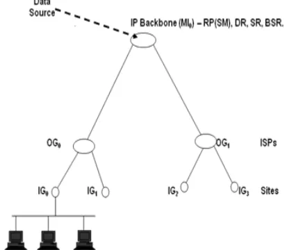
We evaluate the overheads of the protocols in terms of control bandwidth (in byte) consumed to maintain multicast groups on typical networks. In both sparse and dense modes operations on typical hierarchical networks, the overheads of the protocols vary more quickly than the actual data costs for different groups. In dense mode, the flood and prune operation is a global behavior, while in sparse mode, control traffic is constrained along multicast delivery data path trees. Since the links in the networks are assumed symmetrical, we estimate the impacts of the protocols on a typical network in terms of the number of links traversed by control packets. For example, the network in Figure 1 is specified as N(2,2); this means that the network has two branch routers, denoted as m=2,and each of the branch router has two leaf nodes, which is represented as n=2, and N=4 (N is the number of leaf routers in the network). If a data packet, D=1500 bytes, Internet Group Management Protocol (IGMP) control message, C=40 bytes, flood and prune interval, TFP =60 seconds, state refresh time, TSR=60 seconds, and multicast session duration, T=60 minutes, this means that 25 bytes/s (i.e., 0.1953 Kbit/s) of data can be transmitted down the link.
If a multicast group of size, S=2 is given, then we can calculate three different evaluation metrics (e.g., total overhead for the group,TCBOpg , average overhead for the
group, AvCBOpg , and average overhead per group
member, AvCBOpgm ). Using PIM-SM as an example, the number of multicast groups when S=2 are 6 (i.e., 4C2) and the
groups are specified as 0011, 0110, 1100, 1001, 1010, and 0101 [8]. The group, 0011 means that in branch GO0router there is no participating group member while the two group members in GO1 router are actively participating in the multicast session, and data source is outside the network as shown in Figure 1. This implies that IG1 and IG2 site routers
would send two IGPM control packets to OG1 router. The OG1 router would merge the request of the two sites’ routers and sends an IGPM control packet to the IP backbone router (MI0) to establish the delivery data path tree for the group. Following from this, the control cost for this group (0011) is calculated thus;
0011 →3 * C = 3*40 = 120 bytes
Similarly the control costs of the other five groups are; 0110 → 4 * C = 4 * 40 =160 bytes
1100 → 3 * C = 3 * 40 =120 bytes 1001 → 4 * C = 4 * 40 =160 bytes 1010 → 4 * C = 4 * 40 =160 bytes 0101 → 4 * C = 4 * 40 =160 bytes
bytes 880 =
TCBOpg
byte 67 . 146 6 880
=
byte 33 . 73 2
67 . 146
=
= AvCBOpgm
Though, these computed metrics can be used to compare the PIM protocols however, AvCBOpgmis more fine-grained and detailed than TCBOpg and AvCBOpg metrics.
pg
TCBO increases rapidly depending on the number of groups that are generated from a group of size S. AvCBOpgincreases as the size of the group increases, while AvCBOpgmdecreases as the size of the group increases, hence it makes sense to use
pgm
AvCBO metric to evaluate the performance of the protocols. Indeed, if an administration is such that a given amount of bandwidth is allocated to control cost, then
pgm
[image:3.612.49.254.260.440.2]AvCBO can be used for numerical planning to source the most cost-effective multicast protocol for a given network scenario.
Figure 1: A three level Network, specified as N(2,2)
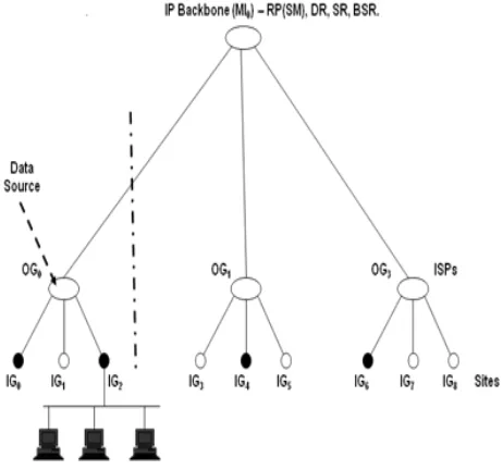
Figure 2: A three level network, data source is outside the network. The network is represented by N(3,3). MI0 is the IP backbone router, OG0, OG1, and OG2 represent different ISPs, while IG0 ... IG8 are sites (stub networks)
with different LAN configurations.
IV. DERIVATIONOFCOSTMODELS
A. Data Source is Outside the Network:
In Figure 2 above, the IP Backbone router (MI0), the branch routers (m), and the leaf routers (N) are labeled level 0, 1, and 2 respectively. When the source router (scr) is outside the network, the cost of the group is a function of the restricted partitions of the group ({si}) (i.e., C=C({si}) [17]. If we know the number of leaf routers in a given group, then we can determine the number not in the group (i.e., N-S), hence the control cost of prune messages depends on the number of group members. In Figure 2, OG0, and OG1 are branch routers with 2 active group members (i.e., IG0 and IG2) in OG1 and 1 active member in OG2(i.e., IG4) respectively. If MI0 router
floods the network as the case in PIM-DM operation, the prune cost associated with OG0 in terms of link count is 1 (i.e., link OG0IG1), while the cost generated by OG1 is 2 links (i.e., OG1IG2, OG1IG5). If the branch routers are swapped, the cost associated with the operation is 3 links. Also, the join cost of the group, in case of PIM-SM protocol is 3 links. If OG1 and OG2 branch routers are swapped, the cost of the group does not change because of the symmetrical nature of the network. It therefore follows that for a three level hierarchical network with data source outside the network, the cost of a group is a function of the partition of the group. This cost is denoted byC{si}.
In Figure 2, the m branch routers (i.e., OG0, OG1, OG2) serve the downstream system routers and their permutation at level one of the network, assuming each branch router has a distinct number of group members is m! However, it is possible for two or more branch routers to have equal number of group members hence we divide the m! by the respective
i
s factorials to avoid the error of double counting in the computation. Following from this analysis, the number of distinct permutations of the m branch routers is
∑
∑= =
× × ×
n j
n o
S jsj
s s s
m
0
1! ... ! !
! . This excludes the permutations of leaf
routers within each branch routers. The arrangement of leaf
routers with s0 members is 0
0
s n
, s1 is 1
1
s n
... snis n s n
n
.
We account for equal number of group members within branch routers by multiplying the number leaf routers in each branch by the respective powers (i.e., si) of the combinatorial factors. Hence, the permutation of the leaf routers within the m
branches is
j s n
j n
j
∏
=
0
. Therefore, the number of multicast
groups subject to the restricted partition S is computed thus,
Q({si}) =
∑
∑
= =× × × n j
n o
S jsj
s s s
m
0
1! ... ! !
!
∏
=
n
j0
j s n
j
(1)
accounts for the arrangements of the leaf routers within the branch routers.
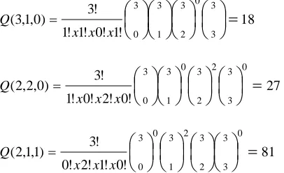
We illustrate the application of this model as follows; as shown in Figure 2, N=9, m=3, n=3, and S=4. The number of
multicast groups in this network is 126
9 4
=
. The restricted
partition of group of size 4 into the 3 branch routers means adding three positive integers from 0,1,...,3 such that the sum of the integers is ≤4. Hence the number of restricted partitions that can be generated are (3,1,0), (2,2,0), and (2,1,1). The partition, (3,1,0) implies that s0=1, s1=1, s2=0, s3=1; (2,2,0)
means that s0=1, s1=0, s2=2, s3=0; and for (2,1,1), s0=0, s1=2,
s2=1,s3=0. The number of multicast groups that can be
generated from these partitions, Q(3,1,0), Q(2,2,0), and Q(2,1,1) is thus;
18 ! 1 ! 0 ! 1 ! 1 ! 3 ) 0 , 1 , 3 ( 3 3 0 3 2 3 1 3 0
=
= x x x Q 27 ! 0 ! 2 ! 0 ! 1 ! 3 ) 0 , 2 , 2 ( 0 3 3 2 3 2 0 3 1 3 0=
= x x x Q 81 ! 0 ! 1 ! 2 ! 0 ! 3 ) 1 , 1 , 2 ( 0 3 3 3 2 2 3 1 0 3 0=
= x x x QFollowing from the above calculation, the number of multicast groups that are generated from the network is 18+27+81=126. This shows that the combinatorial model (1) is accurate. Hence the number of multicast groups for a given network is generated much faster by summing over all restricted partitions than summing over every single group.
If we assume that every group member is equally likely, then the average overhead cost,AvCBO of the groups in a given network is thus;
( )
N s C n j s n j N nj s S s s
m vCBO j j j n j
A
2 } { 1 ! ... ! ! 0 ∏ = ∑ ∑ = ∑ × × =
(2) Where,
2
({
j})
j
s
Q
N j N n j s S∑
∑ =
=
(3)The cost function, C({sj}) includes the cost of linking higher layers that connect the routers to the IP backbone router. For example, the C({sj}) of the PIM-DMFP, written
dmfp i s
C({ }) is specified thus,
∑ + +
= n
i s a C
D s
C({ j}) ( ) i i (4)
Where ai is the link cost , which connects a branch router with sileaf routers to the IP backbone router.
You can recall that the partition, (3,1,0) implies that s0=1,
s1=1, s2=0, s3=1, and the control cost of this configuration in
PIM-MDFP operation is denoted as C(1,1,0,1)and calculated thus, ) 0 0 ) 0 2 ( ) 1 3 )(( ( ) 1 , 0 , 1 , 1
( = D+C + + + + +
C ) ( 6 ) 1 , 0 , 1 , 1
( D C
C = +
SinceQ(3,1,0)=18, the cost control of this partition in a PIM-DMFP operation is,
) ( 108 ) ( 6
18× D+C = D+C bytes
If F({si}) is defined as the probability of restricted partition of a multicast group, then the most general problem to model the average overheads of the protocols is,
( ) ∑ ∑ = ∑ ∑ = = = =
∑
∑
N S s s Q s F s C N S s s Q s F AvCBO S n jj S n jj j j j j j j j 0 0 }) ({ }) ({ } { }) ({ }) ({ (5)If F({sj})is Binomial then,
}) ({ }) ({sj P sj
F = (6)
}) ({sj
P is defined as,
∑
= =
= n
i s P S
P s
P j i i
0 ( )
})
({ (7)
Applying model (7), the weighted average overheads of the protocols is computed by summing over p as,
( )
∑ = ∑ ∑= ∑ = ∑ ∑= = N S nj s S s Q S P s C N S n
j s S s Q S P AvCBO j j j j j j j p 0 }) ({ ) ( } { 0 }) ({ ) ( (8)
The model, (8) holds on the premises that the network is strictly hierarchical, the data source is outside the network, and the overhead cost of the group is a function of the restricted partition of the group.
B. Data Source is Part of the Network:
We have shown in the last section that the overhead cost of a group is a function of Q({sj}) when the data source is outside the network. In this section we establish that when the data source is part of the network the overhead cost of a group depends on Q({sj})and nr(where nris the number of leaf
[image:4.612.38.241.254.378.2]network, hence the overhead cost of a group depends on the partition of the group in the three level network and the nr
members in the two level network.
The more densely populated the two level network (or the more sparsely the three level network) the more cost is involved in setting up and managing a multicast group. This is true, especially for protocols that implement flood and prune mechanism to build and update the delivery data path trees. The data packet used by PIM-DM protocol to flood the network adds significantly to the overhead cost as a result of the huge prune cost in the sparse area of the network. However, the overhead cost can be minimal if the group size is very large.
In both source-rooted and shared-tree protocols, control cost is more involved when the data source is inside the network than when it is outside. This is true for PIM-SM protocol as the data source router builds a unicast short-path tree (SPT) to the RP core router whenever it has data to send to members of the group. The first data packet sent by the data source to the RP router has to be acknowledged by the RP router using a control packet, thus adding significantly to the control cost of establishing and maintaining the group. As the PIM-DM builds its delivery data path tree by flooding the network with a data packet, prune messages are propagated towards the root of the delivery data path tree and the cost of this operation could be so involving for very large networks, especially when the data source is at the lowest level of the network hierarchy.
In Figure 3, the two level network of OG0 branch router has the data source router and the nr local group members while the three level networks of OG1, OG2, and OG3 have group members which are global to the data source router. Then, instead of having a straight-forward combinatorial model as the case of data source outside the network, we now have nr number of combinations. The numbers of nr group members depend on n and S. If the data source is fixed, then nr would run from 0,1,...,n-1 or 0,1,...,S-1 depending on which is minimum (i.e., min(n-1, S-1)). This is true because when the data source sends out data packets, its interface is usually excluded from the receivers’ interfaces except the application is designed to copy the sender for certain reasons.
We calculate the cost of the group in the three level network and then add the cost of the two level network. We denote this cost by C({ }si ,nr). The number of group is
calculated by summing over nr and
(
S−n)
, and then multiply the number of group members in the two level network by the number of group members in the three level network; this result is multiplied by the cost of the group to obtain the total cost of the group. The weighted average overhead cost of the group is obtained by dividing the total group cost by the total number of multicast group in the network.Let the permutation of the (m−1)branch routers of OG1,
OG2, and OG3 be denoted byQ1. Then,
−
=
∑
+
+
×
×
×
−
=
n
r
s
s
o nn
S
s
s
s
m
Q
...
!
!
...
)!
1
(
1 1
1
(9)
Let the permutation of the group members (i.e., leaf routers) in the (m−1) branch routers be denoted by Q2.
Then,
( )
j
s n
j n
j
Q ∏
= =
0
2 (10)
Let the permutation of the nr local group members in the two level networks be Q3. Then,
( )
∑
− −−= =
) 1 , 1 min(
1
0 3
S n
n n n r
r
Q (11)
Thus, by substituting equations (9), (10) and (11) into equation (12), the weighted average overhead cost of the protocols is computed by summing over the probability p as,
(
)
3 2 1
3 2 1
0 ) (
}, { 0
) (
Q N
S
Q Q S P
n s C Q N
S
Q Q S P
AvCBO
r j
p ∑
= ∑
=
= (12)
The above model, (12) holds on the premises that when the data source is inside the network, the overhead of setting up and maintaining multicast groups is a function of the restricted partition of the groups and group members that share the same
branch router with the data source.
[image:5.612.330.561.352.568.2]
Figure 3: A three level network, data source is part of the network.
V. GENERALIZATIONOFTHETHREELEVELS NETWORKPROBLEMS
Algorithm to compute the overhead cost of multicast groups in higher level networks
1. Given a network with parameters, N, L, m, Mk, n, and S; //L, number of levels, m, number of branch routers, Mk (k=0,1,..) number of 3 level networks, n is the capacity of a 3 level network and S the given multicast group in the network 2. While (L≠3); // while network level is not equal to 3 do steps 3 to 9
3. {
4. s=part(S, m, Mk, n); // call a partition function to partition S into m branches such that at most the capacity of each is
m nMk
5. mc=perm(s);// call perm(s) function to permute the partition of s and store result in mc
6. oc=C(s); // call C(s) cost function to compute the overheads of s and store result in oc
7. CBOe +=mc*oc; //sum the overheads of higher levels 8. L=L-1; //decrement network level L by 1
9. }
10.CBO3L=sum (3l);// call the sum(3L) function to get the sum all three level networks using the numerator of model 2 11.TCBO=CBO3L + CBOe; // Total control cost of establishing the delivery data path tree
12. AvCBO TCBON
2
=
VI. COMPUTATIONOFNUMERICALRESULTS
First, we apply model (8) to calculate the impact of the PIM-SM on a fairly small network specified by N(2,3) and our hand-calculated results are shown in Table 1. The results show that the weighted average overhead cost per group member falls as the probability p increases. Following from this, we generate numerical results from fairly large networks using models (8) and (12). The results are computed using C#. We validate our computed results against hand-calculated results to establish the accuracy of our models in evaluating the cost impacts of the protocols in different networks. We set the
probability N S
p= av (where p is the average fraction of
routers in the group) andq=1− p (q is the average fraction of routers not in the group). We set multicast parameters (i.e., multicast session duration T, flood and prune time interval TFP, state refresh time interval TSR) for the different protocol variants and generate results for two network scenarios: data source outside the network and data source is part of the network. We plot average overhead per group member (AvCBOpgm) on the Y-axis against the average fraction of routers for a given multicast group (p) on the X-axis.
The results are shown in Figures 4 to 9. The results are discussed in terms of how the overheads of the protocols vary with different group sizes, the sensitivity of the protocols to different network cardinalities, the responsiveness of the protocols to different sizes of data packets, the location of the
[image:6.612.325.572.105.398.2]data source, and the location of the RP router in PIM-SM operation.
Table 1: Hand-calculated results of Model (8) for PIM-SM performance for fairly small network, N(2,3), data source is outside the network.
Mean (
S
av) p=SavN
AvCBO
pgAvCBO
pgm1 1/6 4445.91 4445.91
2 1/3 8183.53 4091.76
3 1/2 11129.49 3709.83 4 2/3 14215.97 3553.99 5 5/6 16777.62 3355.99
6 1 19200.00 3200.00
0 0.2 0.4 0.6 0.8 1
7 8 9 10 11 12 13 14 15
Average fraction of routers in the multicast group (p)
A
v
C
B
O
per
gr
oup m
em
ber
(
nat
ur
al
l
og s
c
al
e)
Overhead cost performance of the PIM protocols in four level network (data source is outside the network).
SM-4 DMFP-4 DMSR-4 SSM-4
Figure 4: N(3,2,10) network, data source is outside the network, session duration, T= 60 minutes, maximum group is 260.. SM-4, DMFP-4, DMSR-4,
and SSM-4 represent PIM-SM, PIM-DM(FP), PIM-DM(SR) and SSM protocols respectively.
0 0.2 0.4 0.6 0.8 1
9 10 11 12 13 14 15 16 17 18
Average fraction of routers in the multicast group (p)
A
v
C
B
O
per
gr
oup m
em
ber
(
nat
ur
al
l
og s
c
al
e)
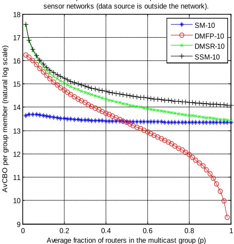
Overhead cost performance of the PIM protocols in hierarchical sensor networks (data source is outside the network).
SM-10 DMFP-10 DMSR-10 SSM-10
[image:6.612.325.561.458.704.2]0 10 20 30 40 50 60 7
8 9 10 11 12 13 14 15 16
Group Size (S)
A
v
C
B
O
per
gr
oup m
em
ber
(
nat
ur
al
l
og s
c
al
e)
Cost behaviour of the PIM protocols in different hierarchy networks
[image:7.612.39.284.64.315.2]SM-L3 DMFP-L3 DMSR-L3 SSM-L3 SM-L5 DMFP-L5 DMSR-L5 SSM-L5
Figure 6: Cost behaviors of the protocols in different network hierarchy. SM-L3, DMFP-SM-L3, DMSR-SM-L3, and SSM-L3 are graphs of three level networks, while SM-L5, DMFP-L5, DMSR-L5, and SSM-L5 are graphs of five level
networks.
0 10 20 30 40 50 60
103 104 105 106 107
Group size (S)
A
ve
rage ove
rhea
d co
st
per
gr
oup m
em
ber
Overhead cost performance of the PIM protocols in different network hierarchies.
SM-L3 DMFP-L3 SM-L4 DMFP-L4
Figure 7: Cost behavior of PIM-SM and PIM-DMFP protocols in different network hierarchies. SM-L3 and DMFP-L3 represent three level networks,
while SM-L4 and DMFP-L4 represent four level networks.
VII. DISCUSSIONOFRESULTS
The overhead cost behaviors of the protocols exhibit similar trends when the data source is outside the networks. The overhead cost per group rises as the mean group increases
(see Table 1), but decreases per group member for all the protocols (see Figure 4). However, when the data source
0 0.2 0.4 0.6 0.8 1
0 50 100 150 200 250 300
Average fraction of routers in the multicast group (p)
A
v
C
B
O
per
gr
oup m
em
ber
(
nat
ur
al
l
og s
c
al
e)
Overhead Cost Analysis of DMFP - Data source outside the network vs data source inside the network.
[image:7.612.332.573.97.347.2]DMFP-Dout DMFP-Din
Figure 8: Comparison of PIM-DMFP protocol, data source outside the network (DMFP-Dout) vs. data source inside the network (DMFP-Din).
0 0.2 0.4 0.6 0.8 1
0 50 100 150 200 250 300
Average fraction of routers in the multicast group (p)
A
v
C
B
O
per
gr
oup m
em
ber
(
nat
ur
al
l
og s
c
al
e)
Overhead Cost Analysis of SSM - Data source outside the network vs data source inside the network.
SSM-Dout SSM-Din
Figure 9: Comparison of SSM protocol, data source outside the network (SSM-Dout) vs. data source inside the network (SSM-Din)
[image:7.612.38.283.369.625.2] [image:7.612.330.576.393.655.2]overhead per group member is plotted against group sizes (see Figure 6). In general, as the mean group size increases the overheads of the protocols narrow down as shown in Figures 4, 6, and 7respectively.
Comparing the protocols, PIM-SM is better than the other protocols in most mean groups (see Figures 4, 6, and 7). PIM-DMSR and PIM-SSM protocols perform very similar for given range of probability. PIM-DMSR protocol appears superior to PIM-SSM except for small mean groups. The reason for this is that as the mean group increases, downstream systems tend to join the group hence more join cost is involved in PIM-SSM than in PIM-DMSR protocol, which involves fewer prune messages as more downstream systems join the group. PIM-DMFP protocol proves to be inefficient over a range of mean groups, except for very large groups (i.e.,Sav→N).
PIM-DMFP protocol appears very sensitive to different levels of network; while the other protocols exhibit similar cost trends (see Figure 5), PIM-DMFP protocols tends to be better than the other protocols when the mean group is above average. This is due to the fact that less overhead is incurred by PIM-DMFP in maintaining its delivery data path trees.
The location of RP router in the network can enhance the performance of PIM-SM protocol (see Figure 7). The performance of PIM-SM is better when RP router is placed at the IP backbone than when it is placed at the ISP (or organization) site. PIM-SM protocol appears sensitive to small mean (or sparse) groups, however as the mean group increases, the average overhead per group member narrows down for the different placements (or locations) of RP router because of averaging effect.
All four protocols perform better in lower level hierarchy networks than higher level hierarchy networks (see Figure 6). This is because as the level of the network increases more control cost is involved in updating (or refreshing) the delivery data path trees.
Comparing the two scenarios, the performances of PIM-DMFP and PIM-SSM protocols are consistently better when the data source is outside the networks (see Figures 8 and 9). Fewer resources are consumed to maintain the delivery data path trees when the data source is outside the network.
These results can be used to determine the flood, join/prune or state refresh intervals, which are usually given as ad-hoc defaults in Internet Engineering Task Force (IETF) documents.
Indeed, if an administration is such that a given amount of bandwidth is allocated to control cost, the relative control costs of the protocols give the relative frequencies with which the distribution trees of the protocols can be refreshed. These findings are significant to the network community; in particular, network administrators can use this information for numerical planning to source the most cost-effective multicast protocol for a given network configuration.
VIII. CONCLUSION
We have demonstrated the application of our generic models in quantifying and analyzing the overheads of the PIM variants in hierarchical networks. We generalize the three
level network problems by giving a simplified algorithm for computing the overheads of the protocols in higher level networks. The models enable us to compute and analyze the overheads of the protocols much faster and efficient in large networks. Analytically, the binomial model is a basic and most simplified assumption. It merely gives equal weight to every group member (leaf router), which may not be the case in real life networks In a real-life network, a multicast router located in a busy area could have more traffic based on the number of end users it serves, and hence would have high probability than a router located in a less busy area, which serves fewer numbers of users. Our future aim is to model this scenario in a real life situation. However, the results of our investigation are very informative and can be used by multicast protocol designers and network integrators to understand in general terms the properties of existing and newly proposed multicast protocols, in particular, how control overheads scale with network configurations. Our analytical models can be used to determine and fine-tune the time intervals for flooding, joining/pruning or state refresh, which are usually given as ad-hoc defaults in Internet Engineering Task Force (IETF) documents
IX. REFERENCES
[1] Alex Bikfalvi, J. García-Reinoso, I. Vidal, F. Valera and A. Azcorra, “P2P vs IP multicast: Comparing approaches to IPTV streaming based on TV channel popularity,” Computer Networks, Vol. 55, Issue 6, Pages 1310-1325, April 2011.
[2] S. Jin and A. Bestavros, “Small-world Characteristics of Internet Topologies and Implications on Multicast Scaling,” Computer Networks, Vol. 50 Issue 5, pp. 648-666, April 2006.
[3] A. Gupta, S. Kalyanaraman, and L Zhang, “Pricing of Risk for Loss Guaranteed Intra-domain Internet Service Contracts,” The International Journal of Computer and Telecommunications Networking, Vol. 50 Issue 15, 2006.
[4] A. Neishaboori and G. Kesidis, “Wireless Mesh Networks based on CDMA,” Computer Communications, Vol. 31 Issue 8, 2008.
[5] F. Filali, H. Asaeda, and W. Dabbous. “Counting the Number of Members in Multicast Communication,” in Proceedings of Networked Group Communication, Fourth International COST264 Workshop, ACM, pp. 63-70, 2002.
[6] T. Bilhartz et al, “Performance of Resource Cost Comparisons for the CBT and PIM Multicast Routing Protocol,” IEEE JSAC, Vol. 15, No. 3, pp. 304-315, 1997.
[7] P. Marbac,“Analysis of a Static Pricing Scheme for Priority Services,” IEEE/ACM Transactions on Networking, Vol. 12, No. 2, pp. 312-325, April 2004.
[8] B. Fenner, M. Handley, H. Holbrook, and I. Kouvelas, “Protocol Independent Multicast - Sparse Mode (PIM-SM): Protocol Specification (Revised,” RFC 4601, 2006.
Mobile IPv6 Networks,” MSWiM’03, Sam Diego, California, USA, September 2003.
[10] A. Bueno, R. Fabregat, P. Vila. “A Quality-Based Cost Distribution Charging Scheme for QoS Multicast Networks”, in Proceedings of the 2nd European Conference on Universal Multiservice Networks, ECUMN'2002, Colmar, France, pp. 268-274, April 2002.
[11] X. Wang, L. Fu, and C. Hu. “Multicast Performance with Hierarchical Cooperation”, IEEE/ACM Transactions on Networking, Issue 99, pp. 1-14, October 2011.
[12] X. Li, S. Tang, and O. Frieder. “Multicast Capacity for Large Scale Wireless ad hoc Networks,” in Proceedings of the 13th annual ACM international conference on Mobile computing and networking, ,September 2007.
[13] C. Hu, X. Wang, and D. Nie, J. Zhao. “Multicast Scaling Laws with Hierarchical Cooperation”, in Proceedings of IEEE, INFOCOM, San Diego, CA, pp. 1-9, March 2010.
[14] F. Zhou, M. Molnar, B. Cousin. “Is Light-Tree Structure Optimal for Multicast Routing in Sparse Light Splitting WDM Networks?” in Proceedings of the 18th International
Conference on Computer Communications and Networks (ICCCN), San Francisco, USA, August, 2009.
[15] H. Liu, “Capacity of Cooperative Ad Hoc Networks with Heterogeneous Traffic Patterns,” in proceedings of IEEE ICC 2011, Kyoto, pp.1-5, June 2011.
[16] A. O¨ zgu¨r, O. Le´veˆque and D. N. C. Tse, “Hierarchical cooperation achieves optimal capacity scaling in ad hoc networks”, in IEEE Trans. Inf. Theory, Vol. 55, No. 10, pp. 3549-3572, October 2007.
[17] J. Akpojaro. “Performance Modelling of Protocol Independent Multicast (PIM) Variants,” PhD dissertation, School of Computer Science and Electronic Engineering, University of Essex, UK, October 2009.
[18] Y. C. Hu and I. Stojmenovic, “Hierarchical Geographic Multicast Routing for Wireless Sensor networks,” Wireless networks, Issue 16, pp. 449-466, 2010.
[19] P. Savola, “Overview of the Internet Multicast Routing Architecture,” RFC 5110, January 2008.