Analysis and Performance Evaluation of Power Amplifier Linearization Techniques

(1)

International Journal of Advanced Research in Computer Science RESEARCH PAPER

Available Online at www.ijarcs.info

Analysis and Performance Evaluation of Power Amplifier Linearization Techniques

Mridula

Research Scholar , ECE Department, Punjabi University, Patiala (Pb)- India

Dr. Amandeep Singh Sappal

Assistant Professor, ECE Department, Punjabi University, Patiala (Pb)- India

Abstract: Linearity performance has become a defining characteristic as it affects power efficiency, channel density, signal coverage, and adjacent

channel power ratio. The non-linearity of Power Amplifier generates inter-modulation (IMD) components, also referred to as out-of-band emission or spectral re-growth, which interfere with adjacent channels. To attain high energy-efficiency, PAs should be operated at their output saturation regions but this operational mode could not provide high bandwidth-efficiency for a single-carrier h igh-order quadrature amplitude modulation (QAM) s ignals a s well a s multi-carrier o rthogonal f requency d ivision multiplexing ( OFDM) s ignals. I t is therefore difficult to co mpensate t he nonlinearity of the power amplifier (PA) in the design of a wireless system. There are several techniques for power amplifier linearization. This paper is based on the mathematical analysis of these linearization techniques and their comparision.

Keywords: Power Amplifier; feedforward linearization; feedback linearization; digital predistortion

I. INTRODUCTION

As the wireless c ommunication is g aining its w idespread popularity, t he i ncreased co mplexity o f t he d evices an d wireless protocols produce an unrelenting neccesity for linear radio f requency ( RF) co mponents an d s ystems. T hese ubiquitous wireless devices r equire h igh p erformance t est systems t o ch aracterize l inearity. Power a mplifiers a re th e important part of the bandpass communication channel system. The s imple p olynomial a pproximation o f nonlinear t ransfer function b ased u pon t he T aylor s eries ex pansion [ 1] can b e used t o d efine t he nonlinear P ower a mplifiers. Typically the odd t erms ar e co nsidered. If ev en-power no nlinear processes are present within the device, there will be variations in the dc conditions. In particular, a device which has significant even-degree distortion will show a low-frequency ac component on its dc supply [2].

II. MATHEMATICAL ANALYSIS OF POWER AMPLIFIER

Power a mplifier d evice n onlinearity ca n b e modeled b y a polynomial

3 5

0( ) 1 i( ) 3 i ( ) 5 i ( )...

V t =a V t +a V t +a V t ₍₁₎

Table1: Coefficients of the intermodulation terms.

Applying a two carrier RF signal to the power amplifier

transistor

( )

cos(

)

cos(

)

in c m c m

V t

=

v

ω

t

−

ω

t

+

v

ω

t

+

ω

t

=

2 cos

v

ω

m

t

cos

ω

c

t

(2)

Where

ω

m

t

represent a mplitude modulation.

ω

c

t

represent carrier waveform

Writing o ut t he r esponse

V t

₀

( )

by pe rforming t rigonometric expansion

3

0 1 3

5 5

( ) 2 cos cos (2 cos cos )

(2 cos cos ) ... (2 cos cos )

m c m c

n

m c n m c

V t a v t t a v t t

a v t t a v t t

ω

= +

+ + + (3)

The De Moivre’s theorem states that

(

)

2 1 2

0

2 1

1

cos

(

)cos 2 1 2

2

n n

n k

n

x

n

k x

k

+

=

+

=

∑

+ −

(4)

for odd powers of cos x, where 1<k< 1/(n-1) Putting e quation ( 4) i n e q ( 3) w e get t he nth d egree o utput

modulated only on fundamental carrier as

Coefficient

order n=3 n=5 n=7 n=9 n=11

Fundamenta

l 9/4 25/4 1225/6

4

3969/6

4 53361/256

3rd_order _{3/4 25/}

8 735/64 1323/32 38115/128

5th_order _- _{5/8 245}

/64 567/32 38115/512

7th_order _- _- _35/

64 567/128 12705/512

9th_order _- _- _- _{63/128 2541/512}

11th_order _231/512

0 1

! 1

( ) 2 ₁ {cos

1 2

2( )!( )!

2 2

!

cos( 2) cos( 2 ) }cos

( )! !

n n

n n m

m m c

n

V t a v n t

n n

n

n n t n k t t

n k k

ω

ω ω ω

−

= ₋ ₊ +

− + −

−

(5)

(2)

Practically, t he f undamental component o f AM-PM d isplays the phase shift

∆

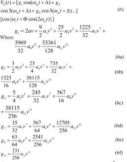
with respect to the AM-AM response. Thus the PA output can be written as

0 1 3

5

( ) [ cos( )

cos3( ) cos5( )...]

[cos{ cos(2 )}]

m

m m

c m

V t g t g

t g t

t t

ω

= + ∆ +

+ ∆ + + ∆

+ Φ

(6)

Where

3 5 7

1 3 5 7

9 11

9

25

1225

2

32

3969

53361

32

128

g

av

a v

=

+

(6a)

3 5 7

3 3 5 7

9 11

3 25 735

2 4 32

1323 38115

16 128

g a v a v a v

a v a v

= + + +

+

(6b)

5 7 9

5 5 7 9

11 11

5

245

567

4

32

16

38115

256

g

a v

=

+

(6c)

7 9 11

7

35

32

7

567

64

9

12705

256

11

g

=

a v

+

a v

+

a v

(6d)

9 11

9 63₆₄ 9 2541₂₅₆ 11

g = a v + a v (6e)

11 11 231₂₅₆ 11

g = a v (6f)

∆

= p hase an gle b /w the AM-AM a nd AM-PM ,

Φ

=peak amplitude of AM-PM d istortion.

ω

_m

t

is t he t wo car rier b eat

frequency which is half of the carrier frequency. The frequency of AM -PM r esponse i s dou ble of t he e nvelope modulation frequency as it has two peaks in every cycle.

Typically t he th ird-order i nter-modulation di stortion pr oduct (IM3) are of most concern since distortion products which are far away in frequency from the desired output can be removed by filtering. B ut typical higher p ower d evices, s uch as LDMOS, which ar e car efully b iased an d t uned i n o rder t o present favorable nulls in the IM characteristics. Such devices shows flat gain characteristics and a very abrupt compression. These devices requires higher order terms, say, up to the ninth order. So from the equation (6) we can find the intermodulation terms as:

3

AM

[ cos3(

m

)]cos

c

IM

=

g

ω

t

+ ∆

ω

t

(7) 1

3

[ cos(

)][

2

(sin(

2

) (sin(

2

)]

PM m

c m c m

IM

g

t

ω

Φ

=

+ ∆

+

−

(8)

5

AM

[ cos5(

m

)]cos

c

IM

=

g

ω

t

+ ∆

ω

t

(9)

2

[

cos(

2)(

)][

2

(sin(

2

) (sin(

2

)]

PM n m

c m c m

IMn

g

n

t

ω

−

Φ

=

−

+ ∆

+

−

(10)

[ cos (

)]cos

AM n m c

IMn

=

g

n

ω

t

+ ∆

ω

t

₍₁₁₎

2

[

cos(

2)(

)][

2

(sin(

2

) (sin(

2

)]

PM n m

c m c m

IMn

g

n

t

ω

−

Φ

=

−

+ ∆

+

−

(12)

Equation (11) and (12) are the generalized equations to find the nth o rder in ter-modulations f or AM-AM a nd AM-PM respectively.

III. LINEARIZATION TECHNIQUES

There are many linearization techniques for minimizing power amplifier nonlinear d istortion. B ut broadly we have f eedback, feedforward and digital predistortion technique for linearization of power amplifier. The following subsections discusses these techniques with their advantages and limitations.

A. RF Feedback

[image:2.595.36.286.104.421.2]

In radio frequency (RF) feedback the output signal is fed back without d etection o r d own-conversion[6]. RF f eedback i s illustrated in Fig 1. The RF signal is input to a subtractor on the left s ide in Fig.1.An a mplifier c an b e used for a n a ctive feedback network or resistors or transformers can be deployed as p assive f eedback n etworks[3]. T he f eedback network can reduce di stortion a ppearing at t he ou tput of t he nonlinear amplifier in Fig1.

Figure 1. RF feedback linearization method

The output of a simple RF feedback circuit is given as

1

AX

Y

A

β

=

+

Voltage-controlled c urrent feedback an d c urrent-controlled voltage feedback ar e co mmonly used as t hey ar e s imple an d their d istortion is p redictable.[4] However, d ue t o t he t ime delays i n t he feedback network, t here i s a dr awback of loop stability pr oblem i n t his de sign. T hus, R F feedback use is limited to narrowband systems.[5]

B.Envelope Feedback

[image:2.595.307.497.361.462.2]

(3)

controlled s uch th at b oth th e in puts o f d ifferential amplifier should r each a t t he s ame t ime. F or t hat t he following expression should follows:

IN PA OUT

[image:3.595.40.281.87.246.2]

∆ = ∆ + ∆

(13)

Figure 2. Envelope feedback linearization.

The attenuator chosen is such that at zero drive voltage there is a cen tered v alue o f at tenuation, s ay

α

₀. T he va lue o f

α

₀ must b e c hoosen to p ermit for s ufficient v ariation o ne o f th e side of t his v alue t o ov ercome a ny gain compression or expansion over the projected operating range.

The attenuator characteristic, at envelope domain time

τ

, can be expressed in the form[2]

0

( ) 1

( (

)

(

))

out VID

in in VID

G V

V

α τ

τ

= +

− ∆ −∆

−

− ∆ − ∆

(14)

Where

∆

outand

∆

inare output and input path delays, respectively. And

∆

VIDis the gain amplifier path delay. The output of main PA can be characterized as

0 1 3

3 5

5

( )

(

))

(

))

(

)) ...

in PA

in PA in PA

V

a

V

a

V

a

V

τ

α

τ

α

τ

α

τ

=

− ∆

+

− ∆

+

− ∆

(15)

Thus if there are more delays and are not controlled, they will obviously generate the non l inear o utput. In o rder t o provide AM-PM co rrection as w ell i n the envelope dom ain f eedback we r equire a method of R F d ifferential p hase d etection. A simple multiplier a s c an b e most e asily r ealized using t he square-law response of a diode.

So if input is

( )

( )co s(

( ))

in m

V t

=

A t

ω

t

+

θ

t

(16)

Then the output will be

0

( ) (1

) ( )co s(

m

( )

)

V t

= −

δ

A t

ω

t

+

θ

t

+

σ

₍₁₇₎

Where

δ

and

σ

are the gain compression and AM-PM at the envelope input level. Thus the output of the multiplier is represented as

( ) (1

) ( ) ( )

cos(

( ))cos(

( )

)

m

m m

V t

A t A t

t

δ

ω

θ

ω

θ

σ

= −

+

1

( )(1

) ( ) ( ){cos

2

cos(2(

m

( ))

A t A t

t

δ

σ

ω

θ

=

−

+

(18)

which will be reduced by the IF filtering to the video signal,

( )

m

V t

=

( )(1

1

) ( ) ( )co s

2

−

δ

A t A t

σ

(19)

A 90o_{phase shifter is required so that phase lead and lag are}

distinguished.

C.RF Power Amplifier Feedforward Linearization

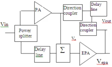
The feedforward linearization technique was invented by H. S. Black [7] a nd a pplied to m any c ommunication s ystems. The feedforward linearization architecture is shown in Fig.3 and it is based on di viding the input signal into two branches. In the main b ranch t he i nput s ignal i s a mplified b y th e main p ower amplifier yielding the PA output [8]. In the second branch the PA output is scaled and compared with the original input.

Figure 3. RF power amplifier feedforward linearization

The resulting error signal goes through a second PA known as the error PA. After the error signal i s obtained it is amplified and added to the delayed output of the main PA. Since the error signal is the nonlinear distortion, adding it from the PA output linearizes the P A. T he following eq uations d escribes the feedforward linearization.

( )

cos

in

V t

=

v

ω

t

and

After passing sampling coupler the output will be 3

1 3

( )

( cos )

pa

V

t

a

v

t

a

v

t

α

=

α

ω

+

α

ω

(20) The input of error amplifier will be

3

1 3

3 3

( )

cos

( cos )

e pa

V t

v

t

V

v

t

a v

t

a v

t

a v

t

ω α

ω

α

ω

α

ω

α

ω

=

−

=

−

= −

if

α

=1/

a

₁

The distortion can be amplified with the auxiliary error PA and added from the original PA output as shown in Fig.3

3

1 3

3 3

( )

( cos )

(1/ )(

( cos ) )

out

V

t

a v

t

a v

t

a v

t

ω

α α

ω

=

+

=

a v

₁

( cos )

ω

t

(21)

which i s l inearized. The g ain o f t he er ror amplifier h as t o b e

greater than 1/α in order to compensate for the (voltage) coupling factor β of the output coupler which is being used to

achieve the necessary addition in the PA output. The output of error amplifier EPA can be written as

3 3

1 3 1 3

3 3

( cos )

(

( cos ) )

epa e e

v

b v

b a v

t

b

a v

t

α

ω

α

ω

=

+

=

+

(22) The transmission coefficient of coupler

γ

is related to coupling coefficient

β

as

γ

=

1

−

β

2 [image:3.595.304.500.176.293.2]

(4)

3

( ) (

)

4

1

(cos )

(cos3 )

4

pa

V

t

a v

t

a v

t

ω

=

+

thus the error amplifier input and output is 3

1

3

( ) [

(

)]cos

4

e

V t

= −

v

α

a v

+

a v

ω

t

3

1 1 3

3 3 3

3 1 3

3

[

(

)]cos

4

3

([

(

)] cos

4

epa

v

b v

a v

t

b

v

a v

t

α

ω

α

ω

=

−

+

−

+

3

1 1 3 3

3 3

1 3

3

[

(

)]cos

4

3

([

(

)] cos

4

b v

a v

t

b

v

a v

t

α

ω

α

ω

=

−

+

−

+

from equation (6) When

α

a

₁=1 then

3 3

3 9

1 3 3 3

3

81

[ {

} {

} ]cos

4

256

epa

b a

b

a

v

= −

α

v

−

α

v

ω

t

(23)

The final output

( )

o pa epa

V t

=

γ

V

t

+

β

v

3 1 3 3

1 3 3 3 9 3 3

3

[ (

)

( {

}

4

81

{

} )]cos

256

b a

a v

v

b

a

v

t

α

γ

β

α

ω

=

+

−

Thus to c ancel th e th ird o rder d istortion we p ut

γ β α

=

b

₁

then the output becomes 3 3

9

3 3

1

81

( ) [

} ]cos

256

o

b

a

V t

=

γ

a v

−

β

α

v

ω

t

(24) Feedforward linearization is stable technique but it suffers from poor efficiency a s an auxiliary er ror PA is required. Feedforward can be used over a wide bandwidth of about 10-100 MHz. However, mismatching of devices in amplitude and phase can lead t o i mpairment an d r educe t he p erformance o f the feedback system. Since this system i s feedforward in nature, al terations i n ag ing an d t emperature d egrade t he correction o f l inearity. T o r educe t hese e ffects, we can u se multiple feedforward loops with a single feedforward loop as the main a mplifier. H owever, th is c onfiguration in creases the complexity of a feedforward system. In a ddition, e xternal devices such as delay lines are necessary.

D. Adaptive Baseband Predistortion

The ad aptive b aseband p redistortion, al so cal led d igital predistortion is b asically a C artesian f eedback with d igital signal p rocessor. T he p rimary d isadvantages o f d igital predistortion is r elative c omplexity a nd b andwidth limitations but it h as accuracy and computational rate of the specific DSP [9]. Furthermore, power consumption is also increased d ue to the digital signal pr ocessor[10]. In a ddition, digital predistortion h as s torage a nd pr ocessing overhead f or t he lookup tables[11].

Fig.4 Adaptive baseband predistortion linearization.

The analysis of predictor w ill be de fined b y f ollowing equations:

( )

( )cos

in

V t

=

v

τ

ω

t

where

τ

is the time in envelope domain '

1 3

3 5

3 5 5

7

7 7

( )

( )co s

( ( )

cos(

))

( ( )cos(

))

( ( )cos(

)) ...

p

V

t

b v

t

b v

t

b v

t

b v

t

τ

ω

τ

ω ϕ

τ

ω ϕ

τ

ω ϕ

=

+

(25)

Using equation (6)

3

1 3 3

5 7

5 5 7

7

3

( )

( )cos

( )cos(

)

4

5

( )co s(

)

35

( )

8

64

cos(

)...

p

V t

b v

t

b v

t

b v

t

b v

t

τ

ω

τ

ω ϕ

τ

ω ϕ

τ

ω ϕ

=

+

(26)

And the PA output will be

' 3 5

1 3 3 5

3

5 1 1 3

5 7

3 5 5 7

3

7 3 1 3

5 7

3 5 5 7

( ) ( ) ( )

3

( )... [ ( )cos ( )

4

5 35

cos( ) ( )cos( ) ( )

8 64

3

cos( )...] [ ( )cos ( )

4

5 35

cos( ) ( )cos( ) ( )

8 64

cos(

o p p p

V t a V t a V t a V

t a b v t b v

t b v t b v

t a b v t b v

t b v t b v

t

ω

ω θ

τ

ω

τ

ω θ

τ

ω θ

τ

ω θ

τ

ω

τ

ω θ

τ

ω θ

τ

ω θ

= + + + + = + + + + + + + + + + + +

+ 3 3

7 5 1 3

5 7

3 5 5 7

5 7

3

)..] [ ( )cos ( )

4

5 35

cos( ) ( )cos( ) ( )

8 64

cos( )..]

a b v t b v

t b v t b v

t

τ

ω

τ

ω θ

τ

ω θ

τ

ω θ

+ +

+ + + +

+

(27)

From the above equation we can extract the third order term as 3

1 3 3 1

3 3

3

[ ( ) co s

(

)

( )

4

cos(

)] ( )

a

b

t

a b

t

v

ω θ

τ

+

In or der t o r emove t hird or der di stortion t he a bove e quation should be zero when

1

a

=

b

₁=1,

b

₃

=

a

₃

/

a

₁ and

ϕ

₃

=

θ π

₃

+

In the similar way fifth order distortion will be null when

3 2

5 5 3 3 3

5 5

5

cos( ) ( )

9

( ) cos 2

9

8

16

8

5

( ) cos

8

b

a

ϕ

θ

=

+

−

and

5

₅

sin( ) ( ) sin 2

₅

9

₃2 ₃

( ) sin

5

₅ ₅

(5)

Thus proper choice of coefficient could remove the distortion in the predistortion technique.

E. Envelope elimination and restoration (EER)

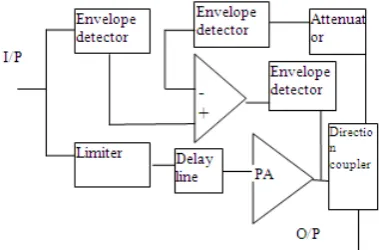
EER i s a t echnique which i ncreases l inearity an d power efficiency simultaneously [12]. The basic method of EER is to split the RF input signal into phase and envelope separately and then combine them after amplification [13]. The basic principle of E ER i s t hat a ny narrow-band s ignal c an be pr oduced by simultaneous amplitude (envelope) and phase modulation. The architecture in Fig.5 shows an EER technique with limiter and envelope detector t o seperate the p hase and envelope information, respectively.

The limiter eliminates the envelope and thus makes it possible for a hi gh-efficient n onlinear P ower Amplifier to a mplify th e constant-envelope signal. Finally, the envelope amplifier creates an a mplified r eplica o f t he i nput s ignal at t he o utput. EER gives better linearity with high

efficiency. H owever, it h as li mited b andwidth o f t he c lass-S modulator a nd th us d ifficulty in correct alignment of th e envelope and phase signals.a jitter or high ACPR could be the issues. Furthermore, high envelope variations can drive the RF power a mplifier in to c utoff a nd th us s ignificant d istortion. However, the resulting feedback poses a problem in bandwidth limitation a nd lo op s tability. F urthermore, c omplexity o f th e circuit i s al so i ncreased. T he modulator is usually a c lass-S amplifier

Figure 5. Envelope elimination and restoration.

IV. CONCLUSION

[image:5.595.310.500.78.203.2]

The l inearization t echniques d iscussed s o f ar has a t radeoff between high ef ficiency, co mplexity an d co st. T he ad ditional circuitry also n eed d elay l ines to c ompensate t he synchronization of multiple inputs. The digital predistorter technique also need additional circuitry and complexity but the efficient adaptive algorithm can be used to give high efficiency power amplifier. A comparison of different RF power amplifier linearization techniques is shown in Table 2.

Table 2. Comparison of different RF power amplifier linearization techniques

Technique Performance Band width

cost Control Drawback

Cartesian Moderate Narrow Moderate Control at input Low gain & stability Polar Moderate Wide Moderate Control at input Low gain

Analog RF

Predistortion Low Wide Low Control at input Comparativily Low gain Digital

Predistortion Moderate Wide Moderate Control at input Easy to control but depends on DSP Feed

forward Good Wide High Control at output Low efficiency

V. REFERENCES

[1] Fadhel M . G hannouchi, O ualid H ammi, M ohamed H elaoui-Behavioral M odelling and Predistortion of W ideband w ireless Transmitters-Wiley, 2015.

[2] Cripps, S teve C. Advanced techniques in RF power amplifier design. Artech House, 2002.

[3] Kenington, P eter B. High linearity RF amplifier design. A rtech

House, Inc., 2000.

[4] D'Andrea, A. N., Lottici, V., & Reggiannini, R. (1996). RF power amplifier lin earization th rough a mplitude a nd p hase predistortion. IEEE Transactions on communications, 44(11), 1477-1484.

[5] Sperlich, Roland, et al. "Power amplifier linearization with digital pre-distortion and crest factor reduction." Microwave Symposium Digest, 2004 IEEE MTT-S International. Vol. 2. IEEE, 2004. [6] Park, H . M ., B aek, D . H ., Jeon, K . I ., & H ong, S . ( 2000). A

predistortion l inearizer us ing e nvelope-feedback t echnique w ith simplified car rier can cellation s cheme for cl ass-A an d cl ass-AB power amplifiers. IEEE Transactions on Microwave Theory and Techniques, 48(6), 898-904.

[7] Black, Harold S. "Inventing the negative feedback a mplifier: Six years of persistent search helped the author conceive the idea “in a flash” aboard the old Lackawanna Ferry." IEEE spectrum 14.12

(1977): 55-60.

[8] Belcher, D onald K ., M ichael A . Wohl, an d K ent E . B agwell. "Feed-forward c orrection l oop with a daptive pr edistortion injection f or lin earization of R F p ower a mplifier." U .S. P atent No. 5,760,646. 2 Jun. 1998.

[9] K .J. M uhonen, M . K avehrad a nd R . K rishnamoorthy, “ Look-up Table Techniques f or Adaptive D igital P redistortion: A Development and Comparison,” IEEE Transactions on Vehicular Technology, vol. 49, no. 5, September 2000, pp. 1995-2002.

[10 Morgan, D . R ., Ma, Z ., K im, J ., Z ierdt, M. G., & Pastalan, J . (2006). A g eneralized memory pol ynomial model f or di gital predistortion of R F pow er a mplifiers. IEEE Transactions on signal processing, 54(10), 3852-3860.

[11] Kim, J., and K. Konstantinou. "Digital predistortion of wideband signals b ased on power a mplifier model w ith m emory."

[image:5.595.41.556.423.556.2]

(6)

elimination and restoration." Proceedings of the IRE 40.7 (1952):

803-806.

[13] Su, David K., and William J. McFarland. "An IC for linearizing RF power amplifiers using envelope elimination and restoration."