Article Design and analysis of the redundancy allocation problem using a greedy technique

Article

Design and analysis of the redundancy allocation

problem using a greedy technique

Souradeep Nanda

_{*, Siddharth Sharma}

_{, Piyush Kundnani}

_{, Anand Shanker Deb}

_{and C.}

1 _{School of Computer Science and Engineering, VIT Chennai, Kelambakkam Road, 600048, Hostel Block A,}

India

2 _{School of Advanced Sciences, Mathematics, VIT Chennai, Kelambakkam Road, 600048, Hostel Block A, India;}

[email protected]

* Correspondence: [email protected]

Abstract

We present a very computationally light and fast approximation algorithm and then verify it with genetic algorithm and simulated annealing. We show that our algorithm is on par with GA and SA in terms of output produced while having a tightly bounded time complexity. Our algorithm works best when there is a strong positive correlation between the reliability of a component and its cost. We present two algorithms with the same essence. One of them is system cost bounded and the other is target reliability bounded. Our proposed algorithm works on a subsystem level redundancy instead of component level redundancy.

Keywords

Redundancy Allocation Problem, Genetic Algorithm, Simulated Annealing, Greedy Algorithm

1.0 Introduction

Machines, factory lines, vehicles etc have a large number of components. Each component can fail at any given time. Reliability of a component is defined to be the chance that a component will be working at a given time.

When a component fails, the whole system may fail. The component then has to be replaced. This is called standby redundancy. In certain situations, say in satellites and probes, we cannot replace a component. Even in power systems and data servers, we cannot afford to bring the entire system down for maintenance. In those cases we use active redundancy. In active redundancy, a server always runs along with all the other servers, when a server fails, it immediately takes over. The model we use in our paper is called binary system reliability framework, which simply means that either the component is

completely working or it has completely failed. There are no intermediate stages.

In either case, we have to have some components or subsystems in our inventory to replace the failed components. The number of components we can have in our inventory can be limited by factors like budget or storage space. The redundancy allocation problem is thus finding a way to maximize reliability while minimizing the cost. This problem has been proved to be NP-Hard by MS Chern [15].

The graph of failure rate of a component over time is said to be bathtub shaped. In most of the component’s lifetime, the failure rate remains constant. Therefore we assume the reliability of the component to be constant.

Figure 1: Bathtub shaped failure rate curve

In order to find the total system reliability, we multiply the reliabilities of each subsystem in series. Here is the reliability of each subsystem in series.

Redundancy at component level is better than redundancy at subsystem level[1] for active redundancy. However it is not true for standby redundancy. [2] In our paper we go for subsystem level redundancy.

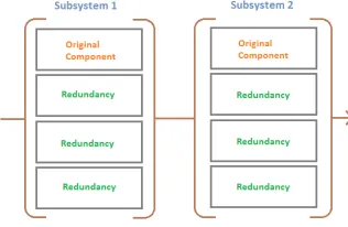
Figure 2: Series parallel redundancy allocation problem

Each subsystem can have different types of components. In this paper we pre-calculate the reliability of all the different types of components and merge it into a single subsystem. Then we go for subsystem level redundancy.

Say we install redundant spares for the subsystem . Then the reliability of this subsystem after installation of redundancies is given as follows.

= 1 − (1 − )

The n vector represents how many redundant spares of each subsystem we have to buy. The total cost of the system then becomes.

= ∑

This problem can be solved using dynamic programming however both space complexity and computational complexity of the DP scheme grow with (∏ ) . Where is the bound of the resource q. [3]

In order to solve the problem faster with less auxiliary space, many scholars have tried using different meta- heuristics. Some scholars have experimented with fuzzy systems [8] and fruit fly optimization techniques [4]. Ant [7] and bee [18] colony optimization techniques can also be used to solve this problem. Artificial immune system algorithms, [9] improved surrogate constraint methods [10] and Tabu search [16] have been successfully implemented as well. [21] have taken into account, the variability data of reliability of components, gathered through field tests. [22] have used an electromagnetism like mechanism to solve the redundancy allocation problem. [23] used a Non-dominated Sorting Genetic Algorithm(NSGA II) after optimizing its operators rate by using Response Surface Methodology (RSM).

In this paper we present a faster method which gives reasonably close results and requires no auxiliary space.

2.0 Cost bounded approach

We claim that the reliability of the system is being limited by the least reliable subsystem. Our claim is in accordance with the law of limiting factors. The concept of limiting factors is based on Liebig's Law of the Minimum, which states that growth is controlled not by the total amount of resources available, but by the scarcest resource. We represent this in mathematical terms using Theorem 1.

Theorem 1: When we multiply n numbers between 0 and 1, the result is always lower than the lowest number.

Proof: We prove it by induction. Let there be n numbers

1

= 1 + 1 + … + 1

First, let us prove it for two numbers.

1

= 1 + 1

=

1 + = 1 +

If > then <

Similarly we can show for >

Using induction, we get

1

( )=

1

( )+

1 + 1

( ) < ( ( ), )

( ) < ( ( ( ), ), )

( ) < ( , , . . . , )

Now, we establish the importance of this law in this context. To minimize the cost, we have to minimize the addition of the numbers in n multiplied by some constants. We maximize the reliability of R by increasing for all i. Increasing would increase . Since is dependent on , we can say that minimizing the summation of will result in minimizing the summation of . is a constant.

Proof: This can be proved using Cauchy’s Mean Theorem

Let there be two numbers x and y. We can write

4 = ( + ) – ( − )

We can see that xy is maximum when − is 0 i.e. = .

Now we extend this proof to n numbers. Let there be two numbers a and b in n numbers such that > and <

for a mean M of the n numbers. Using the above equation we can show that the product of a and b is maximum when = . Since we have chosen a and b arbitrarily, we can repeat the process until all numbers are equal to mean.

In this problem, we are multiplying the reliabilities of each subsystem in series. To have the biggest increase in reliability, we increase the reliability of the least reliable subsystem.

Theorem 3: If we were to maximize the product, we can have the biggest impact by increasing the lowest number in the chain.

Proof: In Theorem 2 we proved that we have to minimize ( − ) for all x and y in n. Say > , now in order to minimize this equation we have to lower x or raise y. Lowering the reliability of a subsystem is not what we are going for, so instead of that, we will increase y to match x. The value of ( − ) grows quadratically as the difference increases. So, we can have the biggest impact on the geometric mean by increasing the reliability of the least reliable subsystem.

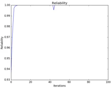
The empirical proof of this claim can be verified by looking at Figure 3 and 4. When we increase the redundancy of the least reliable components, the reliability rapidly increases. After a certain point, the reliability plateaus out.

In the cost bounded approach, we naively increase the redundancy of the least reliable subsystem by one unit. Then we recalculate the reliability of each subsystem including redundancies and the total reliability. This process is repeated until we have exhausted all our available resources. From this process we can see that the less reliable components will be bought more than the more reliable components. Therefore, if the cost of the less reliable components is less than the cost of more reliable components then the resources will be distributed effectively. So our algorithm must take an assumption that the cost and reliability is strongly correlated.

Figure 3: Reliability with respect to number of iterations when there is a strong positive correlation between reliability and cost

Figure 4: Reliability with respect to number of iterations when there is a strong negative correlation between reliability and cost

Comparing figures 3 and 4 we can see that when there is a strong negative correlation, the algorithm stops faster as it has exhausted all its resources.

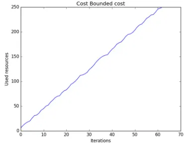
The algorithm is not as fast as the target bounded approach as it consumes the resources linearly as demonstrated from figure 5.

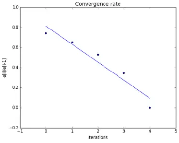
During every iteration, we calculate the reliability of the system. This takes time Θ(n). Then we find the component with lowest reliability, this also takes Θ(n). In the worst case, we have C iterations where C is the cost bound. Therefore the time complexity of this algorithm is O(cn). From empirical analysis (Figure 5) we can say that the convergence rate of this algorithm is super linear.

Figure 6: Convergence rate of cost bounded algorithm

2.1 Target reliability approach

Sometimes, we are more interested in achieving a set level of confidence in terms of reliability rather than exhausting all the available resources. The following algorithm is for those cases.

We fix a target reliability . It is the target reliability of the entire system. In Theorem 2 we have already proved that all the must be equal. Let us call it .

=

=

=

We can now compute , it is the target reliability of each subsystem. Let us call it k. When we equate it with

, we get

1 − (1 − ) = 1 − (1 − )

(1 − ) = (1 − )

Taking log on both sides

(1 − ) = (1 − )

= _{(1 − )}(1 − )

Since ni is integer, we round it up.

= (1 − )_{(1 − )}

This process can be thought as an approximation for integer programming where instead of integer programming, we do linear programming and just round the result. Since the cost has no upper bound in this case, the result is always within the solution space albeit it can be suboptimal, hence it is an approximation. [5] have implemented integer programming techniques to solve problems related with systems reliability design.

This method is similar to using Lagrange Multipliers, implemented by [6].

Just like the cost bounded approach, this works best when the reliability and cost are strongly correlated. Components with less reliability would be bought in far greater quantity then the ones with more reliability.

In figure 7 and 8 we can see that the function converges much faster than the cost bounded approach. This algorithm also has a super linear rate of convergence.

Figure 7: Reliability vs. number of iterations.

Calculating takes constant time. We have to repeat this process for each subsystem. Therefore the time complexity of this algorithm is Θ(n).

2.2 Comparison with Simulated Annealing

Simulated annealing is a probabilistic algorithm. It can be used in a wide variety of applications. The idea behind simulated annealing is derived from the crystallization of metals on cooling. As the crystals cool down, they align into a rigid formation. Simulated annealing interprets slow cooling as a slow decrease in the probability of accepting worse solutions as it explores the solution space. Accepting worse solutions is a fundamental property of meta-heuristics because it allows for a more extensive search for the optimal solution. the method was independently described by Scott Kirkpatrick, C. Daniel Gelatt and Mario P. Vecchi in 1983. [11]

( ) = 1, ( ) > ( )

e ( ) ( ),

P is the probability of transfer to the new state . The function f is the fitness function of a variable x. T is temperature and k is the Boltzmann constant. In the context of redundancy allocation problem, x is the number of redundant components of each subsystem. The fitness function f is the reliability of the system for a given x. We initialize T to be a large arbitrary value and when we set k to be a small value, which is also arbitrary.

The array of the number of components can be thought of a vector whose dot product with the cost vector must be less than or equal to the maximum available resources. In other words, the number of components vector is a direction is hyper dimensional space, scaled up to some constant k, such that the dot product of these vectors is less than equal or to the max cost.

.

For the simulated annealing algorithm, we pick a random unit vector. Then we calculate the constant k using the above formula. We then scale by k and round down each entry to the nearest integer. The result is a count vector whose dot product with the cost vector is less than the maximum allowed cost but very close to it. We can now evaluate the fitness of this vector and run it through the simulated annealing algorithm.

Figure 9: Reliability vs. Iterations of SA, T = 100, k = .01

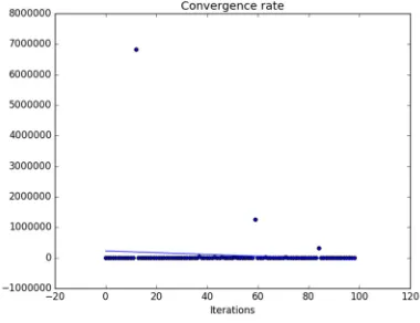
From figure 10 we can empirically tell that our implementation of SA has a linear convergence. The answer given by this simulated annealing algorithm matches with the answers given by our algorithms usually up to three or four digit precision.

Figure 10: SA has a linear convergence.

2.3 Comparison with Genetic Algorithm

Genetic algorithm was originally introduced in 1975 by J. H. Holland [17]. Many researchers already have tried using GA on this problem with many creative approaches and achieved great results. [12] has used a combined neural network and genetic algorithm approach to solve the problem. [13] has studied a bi-objective RAP, which is related to a system of s independent k-out-of-n subsystems in series.

In figure 11 we have the numbers next to the green vectors indicating the number of components and the reliability of the system. The example is only for two dimensions but we can extend the idea to higher dimensions. We can see that all the vectors with the highest reliability are bunched together. Therefore in order to improve reliability, the child must closely resemble the parents. In our crossover function, we interpolate between the parents by a random factor t, in the hope that the child vector would be closer to the solution vector and therefore would have higher fitness than its parents.

[19] had proposed the use of penalty functions in GA, however we do not use it. Instead we just normalize and rescale the vector as done in SA. The GA algorithm does not take into account the length of the vector, only direction is taken into consideration. So it can never exceed the maximum available resources.

Figure 11: The direction of the green vectors represents the number of redundancy of each subsystem 1 and 2. The length represents reliability. The red curve is the first quadrant of a unit circle. Initially the reliability of component 1 and 2 are .7 and .75 respectively. The cost of each component is 2 and 3 respectively and the total available resource is 20.

Figure 12: Reliability vs. Iterations graph of GA

In our mutation function, we apply a random force to each component of the vector in the hope of getting out of any local minima.

Figure 13: Convergence vs. Iterations of GA. Linear convergence is exhibited for most of the iterations.

Conclusion and Future Work

This paper mainly deals with the implementation of redundancy allocation using greedy technique and based on the graphical representations, it reveals the fact that convergence criteria is obtained as a comparative study with genetic algorithm and simulated annealing.

The cost bounded approach increases the redundancy one unit at a time. This is rather inefficient when maximum resource is large and cost of each component is rather small. A more intelligent approach can be devised to solve this problem more efficiently.

The source code used for this research can be found on Github. (https://goo.gl/6DZcdG)

Acknowledgement

Research paper written under mentorship of Dr. C. Vijayalakshmi (VIT Chennai). No funds or grants were provided.

References

[1] Barlow, R. & Proschan, R. (1981). Statistical theory of reliability and life testing, Silver Spring, MD: Madison.

[2] Boland, P. J. & El-Neweihi, E. (1995). Component redundancy versus system redundancy in the hazard rate ordering. IEEE Transactions on Reliability 44, 614–619. [3] Marco Caserta and Stefan Voß (2015). A

[4] Seyed Mohsen Mousavi, Najmeh Alikar and Seyed Taghi Akhavan Niaki (2015) An improved fruit fly optimization algorithm to solve the homogeneous fuzzy series-parallel redundancy allocation problem under discount strategies. [5] Misra KB & Sharma U. An efficient algorithm to

solve integer programming problems arising in system-reliability design. IEEE Trans Reliab 1991 ; 40(1):81–91

[6] Misra KB. Reliability optimization of series-parallel system. IEEE Trans Reliab 1972; 21: 230–8. Zeinal Hamadani A, Akbarzade Khorshidi H. System reliability optimization Using time value of money. IntJ Adv Manuf Technol 2013; 66:97–106(Issue1–4).

[7] Chia LY, Smith A E. Ant colony optimization algorithm for the redundancy allocation problem (RAP). IEEE Trans Reliab 2004; 53(3):417–23.

[8] Seyed Mohsen Mousavi, Najmeh Alikar, Seyed Taghi Akhavan Niaki and Ardeshir Bahreininejad, Professor (2015) Two tuned multi-objective meta-heuristic algorithms for solving a fuzzy multi-state redundancy allocation problem under discount strategies [9] Chen TC, You PS. Immune algorithms-based

approach for redundant reliability problems with multiple component choices. Comput Indus 2005; 56(2):195–205.

[10]Onishi J, Kimura S , James RJW , Nakagawa Y . Solving the redundancy allocation problem with a mix of components using the improved surrogate constraint method. IEEE Trans Reliab 2007; 56(1):94–101

[11]Kirkpatrick, S.; Gelatt Jr, C. D.; Vecchi, M. P. (1983). "Optimization by Simulated Annealing". Science 220 (4598): 671–680

[12]David W. Coit, Alice E. Smith.(1996) Solving the redundancy allocation problem using a combined neural network/genetic algorithm approach

[13]Mehdi Keshavarz Ghorabaeea, Maghsoud Amiria, Parham Azimib (2015) Genetic algorithm for solving bi-objective redundancy allocation problem with k-out-of-n subsystems

[14]A.A. Najafia, H. Karimib, A. Chambaric, Fatemeh Azimid (2013) Two metaheuristics for solving the reliability redundancy allocation problem to maximize mean time to failure of a series– parallel system

[15]M. S. Chern, On the computational complexity of reliability redundancy allocation in a series system. Operation Research Letters, 11,309– 315, 1992.

[16]M. Ouzineb, M. Nourelfath, M. Gendreau, Tabu search for the redundancy allocation problem of homogenous series–parallel multi-state systems, Reliability Engineering and System Safety, 93, 1257–1272, 2008.

[17]J. H. Holland, Adoption in neural and artificial systems. Ann Arbor, Michigan (USA): The University of Michigan Press, 1975.

[18]W.-C. Yeh, T.-J. Hsieh Solving reliability redundancy allocation problems using an artificial bee colony algorithm Computers and Operations Research, 38 (11) (2011), pp. 1465– 1473

[19]D.W. Coit, A. Smith Penalty guided genetic search for reliability design optimization Computers and Industrial Engineering, 30 (4) (1996), pp. 895–904

[20]Aida Karimia, Mani Sharifib, Amirhossain Chambaric (2011) Genetic Algorithm and Simulated Annealing for Redundancy Allocation Problem with Cold-standby Strategy [21]Ali Salmasnia, Ehsan Ameri, Seyed Taghi, Akhavan Niaki (2016) A Robust Loss Function Approach for a Multi-Objective Redundancy Allocation Problem

[22]Mohammad Teimourib,Arash Zaretalaba,S.T.A. Niakic,Mani Sharifib (2016) An efficient memory-based electromagnetism like mechanism for the redundancy allocation problem

[23]M. R. Shahriari (2016) Set a bi-objective redundancy allocation model to optimize the reliability and cost of the Series-parallel systems using NSGA II problem