Translucent Voices: Creating Sound Pedagogy And Safe Spaces For Transgender Singers In The Choral Rehearsal

(1)

University of South Carolina

Scholar Commons

Theses and Dissertations

2018

The South Carolina Safety Belt Study: Large-Scale

Location Sampling

Stephanie Jones University of South Carolina

Follow this and additional works at:https://scholarcommons.sc.edu/etd Part of theStatistics and Probability Commons

This Open Access Dissertation is brought to you by Scholar Commons. It has been accepted for inclusion in Theses and Dissertations by an authorized administrator of Scholar Commons. For more information, please contactdillarda@mailbox.sc.edu.

Recommended Citation

Jones, S.(2018).The South Carolina Safety Belt Study: Large-Scale Location Sampling.(Doctoral dissertation). Retrieved from

(2)

THE SOUTH CAROLINA SAFETY BELT STUDY: LARGE-SCALE LOCATION

SAMPLING

by Stephanie Jones Bachelor of Science University of Denver, 2016

Submitted in Partial Fulfillment of the Requirements For the Degree of Master of Science in

Statistics

College of Arts and Sciences University of South Carolina

2018 Accepted by:

John Grego, Director of Thesis Wilma Sims, Reader Brian Habing, Reader

(3)

ii

(4)

iii

ABSTRACT

The South Carolina Safety Belt Study is a statewide survey completed yearly to assess the prevalence of safety belt usage on of South Carolina roads through

observations from different locations across the state. Every five years the sites for

(5)

iv

LIST OF TABLES

Table 3.1 Statewide Highway Data ...11

Table 3.2 Statewide Other Data ...12

Table 3.3 Census Bureau Data ...13

Table 3.4 Statewide Traffic Points Data ...14

Table 3.5 Strata Data...15

Table 5.1Aiken Sampled Road Reaches ...23

Table 5.2 Anderson Sampled Road Reaches ...24

Table 5.3 Charleston Sampled Road Reaches ...25

Table 5.4 Cherokee Sampled Road Reaches ...26

Table 5.5 Colleton Sampled Road Reaches ...27

Table 5.6 Darlington Sampled Road Reaches ...28

Table 5.7 Dorchester Sampled Road Reaches ...29

Table 5.8 Greenville Sampled Road Reaches ...30

Table 5.9 Horry Sampled Road Reaches ...31

Table 5.10 Lexington Sampled Road Reaches ...32

Table 5.11 Oconee Sampled Road Reaches ...33

Table 5.12 Orangeburg Sampled Road Reaches...34

Table 5.13 Spartanburg Sampled Road Reaches ...35

Table 5.14 Sumter Sampled Road Reaches ...36

(7)

vi

(8)

1

CHAPTER 1 INTRODUCTION

Across the country, the past two decades have seen a gradual increase in safety belt usage. The National Highway Traffic Safety Administration (NHTSA) estimates the national seat belt use rate, defined as being restrained by a shoulder-style belt, has jumped from 79.9% in 2000 to 90.1% in 2016 (Li and Pickrell 1). This increase is important, because it has also been accompanied by steady decrease in the percentage of daytime unrestrained passenger vehicle occupant fatalities from 51.6% in 2000 to 40.7% in 2016 (Li and Pickrell 1). This association in conjunction with research that shows a reduction of risk for fatal injury by 45% with the use of a safety belt makes their usage rate a serious focus of state governments to protect their constituents (Li and Pickrell 4).

(9)

2

the existence of the SC law, many people in South Carolina do not use appropriate safety belts when behind the wheel. A survey conducted by the Department of Statistics in June 2008 found the usage rate for shoulder-style belts to be 79% (Grego 3). Even with the benefit of being a primary law state, this is lower than NHTSA’s nation-wide 2008 estimate of 83.1% (Li and Pickrell 1). There is a need for further education and

awareness of the benefits of seatbelts in South Carolina until usage rates approach 100%.

Since May of 1991, the office of Highway Safety of the South Carolina

Department of Public Safety has created a safety belt awareness drive and commissioned the Statistical Laboratory at the University of South Carolina (Stat Lab) to survey to assess the success of their campaigns (Grego 4). While the commissions were sporadic for a period, they were completed for the years 1991, 1992, 1993, 1994, 1995, 1998, 1999, and every year since there has been a survey before and after the drive to assess the success of it (Grego 4).

To complete this survey individual people who observe motorized vehicles at each location (counters) are sent to specific road locations in the state and record their observations for an hour. For each observation the counter records the type of vehicle, gender of the person, ethnicity of the person, position of the person, and use of seatbelt (Grego 7). Every five years these road locations that are used by the counters are

(10)

3

CHAPTER 2 METHODS

The sample of specific road locations must be chosen randomly, but there are ways of randomly sampling which would provide a more desirable random sample than simply selecting 192 road reaches from all of South Carolina. Thus, a couple other factors were considered when designing the sampling in addition to randomness. First, taking the size of the state of South Carolina into consideration, it makes sense that each of the chosen road samples should be relatively close to some group of the other road samples to cut down on travel time. Next, the sample should be a good representation of the different areas of the state as different areas are vastly dissimilar in terms of variables that contribute to safety belt usage. Finally, it must be considered that funding is limited. Therefore, the sample must comprise different representative parts of the state, as sampling the entire state would not feasible within a reasonable budget.

(11)

4

and Notz 70). Most complex sampling can be done with these methods or some combination of these methods based on the requirements of the survey. For example, cluster sampling is often used at the last step in location sampling, so the chosen individuals to be surveyed are in close proximity to each other (Moore, and Notz 70). This minimizes the cost of on-location sampling both in time and labor.

Bearing in mind all the previous considerations, a specific sampling scheme was developed by the Stat Lab for this survey. Its refinement in 2003 is still the current method used (Grego 13). Initially, to guarantee the sample is representative, the state is broken down into six different strata. Counties are classified as “upstate,” “midlands,” or “lowcountry” based on their geographical region (Grego 5). Then each county is

classified as either “rural” or “urban,” where at least 50% of the population being classified as urban makes the county urban (Grego 5). The combination of these classifications leads to the six strata: upstate rural (UR), upstate urban (UU), midlands rural (MR), midlands urban (MU), lowcountry rural (LR), and lowcountry urban (LU). Then 16 counties are chosen proportionally to their size based on their average daily traffic intensity, where the number of counties per strata sampled is also proportional to their average daily traffic intensity versus the average daily traffic intensity across the state (Grego 5). The variable used to account for these weights was the vehicle miles traveled (VMT). This ensures the sample is representative of traffic across the entire state of South Carolina. Once the counties are selected, four census tracts are randomly

(12)

5

need to cut time and labor cost. From the census tracts, two major road sections and one minor road section were sampled using a SRS. These road sections are where the counters will observe for the survey. The process for the sampling is certainly more complicated than taking a simple random sample, but the stratification captures the considerations of the study while preserving the randomness.

Each road section in South Carolina (that is included in the data for the population for the survey) ends up with a distinct probability of being selected that is the product of the probability of their county being chosen, the conditional probability of their census tract being chosen within each county, and the conditional probability of the specific road section being chosen within each census tract. This “probability of intersection k in tract j in county i in stratum s being included in the multistage sample” can be represented as πsijk (Grego 17). This is just the product of the distinct probability of the county being

(13)

6

CHAPTER 3 THE DATA

There is not a single data source that appropriately contains the entire population for the sample. Further, the stratification of the population necessitates appropriate data sources to define the strata. Therefore, the data used to complete the sampling came from four original datasets. The original datasets are produced by the specified departments within the state of South Carolina and are publicly available. There was also a dataset created by hand to attach the strata information.

The first dataset is a collection of reaches of the statewide highways in South Carolina as a Shapefile for ArcGIS. Shapefiles include the geographical location of data. These are part of the population of road sections. This dataset is called Statewide

(14)

7

END_MILEPO is an integer representing the ending mile post. The variable ROUTE_ID is the name of the highway the reach is a part of, for example “ALLENDALE S-111 N.” The variable FEATURE_TY gives more information on which feature of a highway this is, like “I_Ramp.” The variable MSLINK is a numeric identification code ranging from 457077 to 865627. The variable STREET_NAM includes the name of the street, i.e. “CROOKED CREEK RD.” All of these variables, aside from MSLINK and

COUNTY_ID, may or may not be available for each road section. Therefore, there is a lot of missing data.

The second dataset is similar to the statewide highways dataset, but instead includes stretches from non-highway roads. The SC DOT calls these roads “other,” and they make up the rest of the population of road sections. This dataset is called Statewide Other. The key variables’ first 20 observations are included in Table 3.2. The Shapefile’s associated DBF includes 248,547 rows and 36 variables. Most of these variables coincide with the variables in the statewide highway database. The notable exception is that the numeric identification code variable MSLINK is replaced with the variable ID, which ranges from 283167 to 972825. While these variables are slightly different, they both serve the same purpose of identifying the road section. Neither of the key variables in this dataset contain missing values.

(15)

8

numeric digits 1 through 46. The second is the variable TRACTCE, which attaches the census tract to each observation. There are no missing values in this dataset.

The fourth dataset is a Shapefile of Statewide Traffic Points that has the information for the average daily traffic intensity that is needed for the weights of the samples. The key variables’ first 20 observations are included in Table 3.4. The Shapefile’s associated DBF includes 11,539 rows and 11 variables. There are four variables that were used. The variable CountyName identifies the county the traffic point is in using the complete name, such as “ABBEVILLE.” The variable FactoredAA gives the average daily traffic intensity. The variable Latitude lists the latitude of the traffic point. The variable Longitude lists the longitude of the traffic point. While this file contains detailed information on the traffic intensity, its only location identifying variables are Latitude and Longitude. These variables do not match the specific road reaches from the Statewide Highway and Statewide Other files. Therefore, the combination of datasets are needed. The Statewide Highway and Statewide Other datasets comprise the sampling pool with location information, while the Statewide Traffic Points create the weights. The Census Bureau dataset is needed to match census tracts to the other datasets.

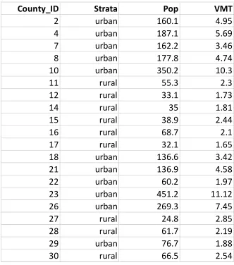
Finally, a small dataset was created by hand to attach strata information to the datasets. It is referred to as ccode29. The key variables’ first 20 observations are included in Table 3.5. It has 29 rows and 4 variables. The variable County_ID is a numeric

(16)

9

There are only 29 counties, as some counties will be removed from the sampling pool, which is explained in the next chapter. This dataset has no missing data and was compiled by information from the South Carolina government.

Each of the Statewide Highway, Statewide Other, and Statewide Traffic Points datasets needed to be joined with the census tracts from the Census Bureau dataset. To do this, they each needed a variable to match on. The Census Bureau had a clear COUNTY variable to match on, so all that was needed was a matching variable in the three datasets. For Statewide Highway and Statewide Other the COUNTY_ID variable was already in a matching format. For Statewide Traffic Points, however, the variable CountyName contained the appropriate information but in a different format. Therefore, some quick SAS code was written to create a variable with this information that was in the same numeric form.

(17)

10

(18)

1

Table 3.1 Statewide Highway Data

COUNTY_ID ROUTE_TYPE ROUTE_NUMB ROUTE_DIR BEG_MILEPO END_MILEPO DATA_SOURC ROUTE_ID FEATURE_TY MSLINK STREET_NAM

3 S- 275 N 0.05 0.1 ALLENDALE S-275 N City_Paved_Sec 458601 HILL ST

25 S- 110 E 0.2 0.36 SCC HAMPTON S-110 E City_Paved_Sec 459599 MIDDLE ST

25 S- 110 E 0.73 0.78 SCC HAMPTON S-110 E City_Paved_Sec 459602 WOOD ST

3 S- 112 E 0.24 0.31 ALLENDALE S-112 E City_Paved_Sec 459603 LEE AVE S

3 S- 112 E 0 0.12 ALLENDALE S-112 E City_Paved_Sec 459606 LEE AVE N

3 S- 111 N 0 0.07 ALLENDALE S-111 N City_Paved_Sec 459607 BEAUFORT AVE N

3 S- 111 N 0.07 0.13 ALLENDALE S-111 N City_Paved_Sec 459608 BEAUFORT AVE N

3 S- 111 N 0.13 0.2 ALLENDALE S-111 N City_Paved_Sec 459609 BEAUFORT AVE N

3 S- 105 N 0 0.17 ALLENDALE S-105 N City_Paved_Sec 459610 COTTON ST W

3 S- 105 N 0.17 0.2 ALLENDALE S-105 N City_Paved_Sec 459611 COTTON ST W

3 S- 105 N 0.2 0.41 ALLENDALE S-105 N City_Paved_Sec 459612 COTTON ST W

3 S- 106 E 1.21 1.4 ALLENDALE S-106 E Paved_Sec 459613 BETHEL CHURCH RD

3 S- 106 E 0 1.21 ALLENDALE S-106 E Paved_Sec 459614 BETHEL CHURCH RD

3 S- 123 N 0 0.06 ALLENDALE S-123 N City_Paved_Sec 459881

25 S- 114 E 0.37 0.43 SCC HAMPTON S-114 E City_Paved_Sec 459968 THIRD ST

(19)

1

2

Table 3.2 Statewide Other Data

COUNTY_ID ROUTE_NUMB STREET_NAM ROUTE_TYPE ID BEG_MILEPO END_MILEPO ROUTE_ID ROUTE_DIR

46 4463 SHADOW LAWN CT L- 964710 0.178 0.25 L-4463 N

46 4460 SHADE TREE CIR L- 964708 0 0.244 L-4460 E

26 1030 GRAINLOYD RD L- 688301 0 0.343 L-1030 E

26 6472 S OAK ST L- 688302 0 0.071 L-6472 E

26 6472 S OAK ST L- 688303 0.071 0.138 L-6472 E

26 6472 S OAK ST L- 688304 0.138 0.203 L-6472 E

26 3374 CHAPIN CIR L- 688305 0.165 0.376 L-3374 E

1 354 BOWERS RD L- 284740 0 0.107 L-354 E

26 3374 PINENEEDLE DR L- 688306 0 0.064 L-3374 E

26 6473 LUMBER ST L- 688307 0 0.073 L-6473 N

26 6473 LUMBER ST L- 688308 0.073 0.096 L-6473 N

26 4045 CANAL ST L- 688309 0 0.025 L-4045 N

26 6474 CLUB CIR L- 688310 0 0.043 L-6474 E

26 4824 ANTIGUA DR L- 688311 0.173 0.239 L-4824 E

1 1464 THREE B DR L- 284747 0 0.241 L-1464 E

46 5409 SHADOW COVE LN L- 964709 0 0.073 L-5409 N

46 2117 SHADOW LAKES DR L- 965301 0 0.407 L-2117 N

46 2327 STATEVIEW BLVD L- 965303 0.055 0.65 L-2327 N

46 1726 TILLMAN ST L- 965302 0 0.088 L-1726 E

(20)

13 Table 3.3 Census Bureau Data

STATEFP COUNTYFP TRACTCE

45 003 020701

45 003 021500

45 007 011001

45 007 012001

45 013 002101

45 013 010900

45 015 020401

45 015 020716

45 019 000200

45 019 000600

45 019 002606

45 019 003600

45 019 004613

45 019 004902

45 019 005100

45 027 960202

45 027 960701

45 031 010100

45 031 011200

(21)

14 Table 3.4 Statewide Traffic Points Data

CountyName FactoredAA ID1 Latitude Longitude

ABBEVILLE 2300 1 34.193697321731 -82.4014862711541

ABBEVILLE 2500 2 34.196450286258 -82.3973930972611

ABBEVILLE 4800 3 34.4197913120729 -82.3852145519501

ABBEVILLE 5000 4 34.3834395735549 -82.3532441946332

ABBEVILLE 3700 5 34.3709915050999 -82.3376546721275

ABBEVILLE 6600 6 34.1788869315088 -82.3801676355446

ABBEVILLE 2400 7 34.1836865592899 -82.3811426013754

ABBEVILLE 2300 8 34.1858833719841 -82.3809593065369

ABBEVILLE 2100 9 34.1896689411347 -82.3826814283596

ABBEVILLE 2300 10 34.1952658266384 -82.3853382522971

ABBEVILLE 3700 11 34.2209709723427 -82.3895787634777

ABBEVILLE 2200 12 34.2321243575607 -82.3904430145627

ABBEVILLE 1600 13 34.2988494874448 -82.3722809521678

ABBEVILLE 1500 14 34.3262312257558 -82.3782540467296

ABBEVILLE 2000 15 34.3330047879849 -82.3873267589961

ABBEVILLE 1600 16 34.3344286550853 -82.402000901482

ABBEVILLE 750 17 34.3886218878848 -82.4367017598433

ABBEVILLE 1850 18 34.0610125382176 -82.3761504017796

ABBEVILLE 2600 19 34.1425013928865 -82.3879748823615

(22)

15 Table 3.5 Strata Data

County_ID

Strata

Pop

VMT

(23)

16

CHAPTER 4 SAMPLING

After the Statewide Highway, Statewide Other, and Statewide Traffic Points had the census tracts joined, they were ready to be sampled. First, the Statewide Highway and Statewide Other datasets were joined together in SAS to create one dataset named All that contains the entire population of road reaches to be sampled. In an attempt to create a distinct identification variable in this new dataset, the variable MSLINK from Statewide Highway had 250,000 added to each value. This number was chosen as there were 248,547 observations in the other dataset, so this comes from rounding this number up. This new MSLINK and the Statewide Other variable of ID were combined to make a new identification variable ObjectID. Therefore, the dataset All had the variables

COUNTY_ID ROUTE_TYPE ROUTE_NUM ROUTE_DIR BEG_MILEPO

END_MILEPO ROUTE_ID FEATURE_TY, STREET_NAM TRACTCE, and the new variable, ObjectID.

Before sampling All had some undesirable observations removed. Due to a request from the National Highway Traffic Safety Association, counties that were deemed to have too few county traffic fatalities were removed using the COUNTY_ID variable. The NHTSA provided a cumulative traffic fatality threshold of 85%, and counties above this were removed. These counties were Abbeville, Allendale, Bamberg, Barnwell, Calhoun, Chesterfield, Edgefield, Fairfield, Greenwood, Hampton, Lee,

(24)

17

a “not in” statement in SAS. There were also observations that were undesirable to be sampled based on the type of road they came from. Roads that were s-ramps, private, or unpaved were all removed from the sample with “not in” statements in SAS.

Additionally, road reaches that did not have a census tract were removed, as they could not be sampled using the current sampling scheme. The last thing done to All was

creating a variable roadtype classifying observations with route-type beginning with “L-“ as “Minor,” as these were local roads. All other observations were classified as “Major.”

Before sampling, the dataset from Statewide Highway Traffic Points also needed to be cleaned up. This data was read into a SAS dataset called Tract16. The issues with making Tract16 ready to be sampled were more complex to fix. For each census tract, two major roads and one minor road needed to be available to be sampled. However, many census tracts did not comply with these counts. Specifically, may did not have at least two major roads. To remedy this problem each nonconforming census tract was looked up in ArcGIS and joined to another census tract based on its location. If multiple problem tracts could be combined to meet the requirement, this was given preference. If not, the census tract was matched with the closest census tract that was conforming. Proc Freq and Proc Sql were utilized to identify the problem tracts and exported to Excel where the new assignment of census tracts was recorded. After all revisions were

(25)

18

with less than one major road from Proc Sql not including observations with values of zero. In the future, this should all be performed in one step.

To sample the counties the ccode29 file had two calculated variables added. The first is sumvmt which collects the sum of the VMT for the strata for each observation. The second is vmtprop which is the proportion of the VMT which is calculated by dividing the individual county’s VMT by its strata’s sum VMT. This was exported under the name CountyWeights.txt and read into R. In R the counties were selected randomly with respect to their weights as described in Chapter 2. They were then output with their respective probabilities of being selected (computed from their vmtprop). The counties selected were Aiken, Anderson, Charleston, Cherokee, Colleton, Darlington, Dorchester, Greenville, Horry, Lexington, Oconee, Orangeburg, Spartanburg, Sumter, Williamsburg, and York. Then All and Tract16 were narrowed down to only observations in these selected counties.

(26)

19

and calculations steps are completed three times, so there are backup samples in case the counters are unable to survey in a location.

To finish up the road sections were sampled. To do so R is again utilized. First some cleaning must be done in R to run the functions: the census tract codes were padded with zeros, as some county codes were shortened by a single digit, and the county and census tract probabilities needed to be rounded. Sampling pools of Major roads and Minor roads also had to be made for each of the sampled census tracts. After this a simple random sample of one Minor road and two Major roads from each census tract was taken, giving 192 total distinct road reaches. The probability of each road sample within its census tract was calculated as one divided by the total number of either Major or Minor roads in the respective census tract. This probability was also multiplied by the county and census tract probabilities to get the total probability of the sampled road reaches. This is exported as RoadSamp.txt and read into SAS. There are also two other copies of this sampling done in case the counters encounter bad locations in the sample.

These sampled road reaches are read back into SAS where they are matched with the All dataset to get the location information needed to give to the counters. This match is done with the variables RoadSamp and ObjectID. After this match is done, however, an issue became obvious: some roads were being matched to the wrong road from the All dataset. The reason for this turns out to be overlapping ID variable values in the

(27)

20

own “ObjectID” variable for each record. This would be distinct and sure to start from one. This should have been utilized for identifying Statewide Other’s records, and this same ObjectID variable, plus 250,000, should have been utilized for identifying Statewide Highway’s records. Once this was corrected, however, the rest of matching went smoothly, and location data was added to the sample.

(28)

21

CHAPTER 5 RESULTS

The final sample is featured in Tables 5.1 to 5.16 separated by county. It has a total of 192 road reaches, 128 major roads, 64 minor roads, 64 distinct census tracts, and 16 distinct counties.

(29)

22

in their personal GPS and feel confident that they are arriving at the correct location. An example of these maps is included in Appendix E.

In April 2018 a smaller scale pre-survey will be completed with the new locations. Only six counties will be surveyed to keep costs down. To ensure this sample is still representative, each strata was sampled, one county was selected from each of the strata: UU, UR, MU, MR, LU, LR. To do this sampling SRS was used. This is

(30)

2

3

Table 5.1 Aiken Sampled Road Reaches

Strata Code County Tractc RoadSamp RoadType CountyProb TractProb RoadProb Prob GPS Coordinates

(31)

2

4

Table 5.2 Anderson Sampled Road Reaches

(32)

2

5

Table 5.3 Charleston Sampled Road Reaches

(33)

2

6

Table 5.4 Cherokee Sampled Road Reaches

(34)

2

7

Table 5.5 Colleton Sampled Road Reaches

(35)

2

8

Table 5.6 Darlington Sampled Road Reaches

(36)

2

9

Table 5.7 Dorchester Sampled Road Reaches

(37)

3

0

Table 5.8 Greenville Sampled Road Reaches

(38)

3

1

Table 5.9 Horry Sampled Road Reaches

(39)

3

2

Table 5.10 Lexington Sampled Road Reaches

(40)

3

Table 5.11 Oconee Sampled Road Reaches

(41)

3

4

Table 5.12 Orangeburg Sampled Road Reaches

(42)

3

5

Table 5.13 Spartanburg Sampled Road Reaches

(43)

3

6

Table 5.14 Sumter Sampled Road Reaches

(44)

3

7

Table 5.15 Williamsburg Sampled Road Reaches

(45)

3

8

Table 5.16 York Sampled Road Reaches

(46)

39 Table 5.17 April Small Sample

Strata

Code

County

UU

4 Anderson

UR

37 Oconee

MU

32 Lexington

MR

38 Orangeburg

LU

10 Charleston

(47)

40

CHAPTER 6 CONCLUSION

Now that the sample has been produced it will remain in use for the next five years until it is resampled in 2023 (barring any changes to the historical application of the survey). First, the survey for April 2018 will be conducted with the smaller sample of six. Then in June 2018 the entire sample of sixteen will be conducted. Data will be analyzed after this survey, and after each subsequent year’s two samples (Grego 4).

In the future, sampling could be simplified with some minor changes. Most importantly the variable ObjectId should be used as the identification code variable instead of MSLINK and ID. This would prevent the issue that arose of mismatched data due to identification variables overlapping in the Statewide Highway and Statewide Other Roads datasets. Secondly, addressing the issue of numeric variables being read in

inconsistently as both numeric and character should be done prior to any analysis. It is easy to lose track of records with a dataset of this magnitude in SAS without immediately noticing. Further, it is not suggested to match on numeric variables in SAS. This presents a problem if County is numeric as it is necessary to simplify multiple datasets down to only those that include the sampled counties, for instance removing counties with less than the NHTSA’sthreshold for traffic fatalities .

(48)

41

more warranted, as South Carolina nears the nationwide 89.7% usage (Li, and Pickrell 1). Comparisons between roads with low speed limits, like the dirt roads and mall parking lots that were eliminated from this study, and roads with higher speed limits may be more important as awareness increases. The focus could also shift to motorcycles, which while currently studied were not included until 2006 (Grego 7). As less motorcycles are

(49)

42

REFERENCES

"South Carolina Department Of Public Safety". Buckleupsc.Com, 2013, http://www.buckleupsc.com/seat_belt_law.asp. Accessed 13 Mar 2018.

Grego, John. South Carolina Statewide Survey Of Safety Belt Use: June 2008.

Department Of Statistics At University Of South Carolina, Columbia, SC, 2008, pp. 3-20, http://www.scdps.gov/oea/attachments/SafetyBelt_Report_2008.pdf. Accessed 13 Mar 2018.

Li, R., and T.M. Pickrell. Seat Belt Use In 2017—Overall Results. National Highway Traffic Safety Administration, Washington, DC, 2017, pp. 1-4,

https://crashstats.nhtsa.dot.gov/Api/Public/Publication/812465. Accessed 13 Mar 2018.

Moore, David S., and William I. Notz. Statistics: Concepts and Controversies. 8th ed., W.H. Freeman and Company, 2012.

“Spatial Join.” ArcGIS for Desktop, ArcMap,

desktop.arcgis.com/en/arcmap/10.3/tools/analysis-toolbox/spatial-join.htm.

(50)

43

APPENDIX A

R CODE: FUNCTIONS FOR SAMPLING COUNTIES

ADAPTED FROM STATLAB 2003

funct.2<-function(Nh,p){ ## for sampling two counties from strata n<-Nh

pii<-rep(0,n) ## create and assign weights for(i in 1:n){

sumj<-0 for(j in 1:n){ if(j!=i){

sumj<-sumj+p[j]/(1-p[j]) }

}

pii[i]<-p[i]*(1+sumj) }

pii }

funct.3<-function(Nh,p){ ## for sampling three counties from strata n<-Nh

(51)

44 for(i in 1:n){

sumj<-0 for(j in 1:n){ if(j!=i){ sumk<-0 for(k in 1:n){ if((k!=i)&(k!=j)){

sumk<-sumk+p[k]/(1-p[j]-p[k]) }}

sumj<-sumj+p[j]*(1+sumk)/(1-p[j]) }}

pii }

funct.4<-function(Nh,p){ ## for sampling four counties from a strata n<-Nh

pii<-rep(0,n) ## create and assign weights for(i in 1:n){

(52)

45 sumk<-0

for(k in 1:n){ if((k!=i)&(k!=j)){ suml<-0

for(l in 1:n){

if((l!=i)&(l!=j)&(l!=k)){

suml<-suml+p[l]/(1-p[j]-p[k]-p[l]) }}

sumk<-sumk+p[k]*(1+suml)/(1-p[j]-p[k]) }}

sumj<-sumj+p[j]*(1+sumk)/(1-p[j]) }}

pii

## creating sample using weights

Sprob1=funct.2(length(strata.name[strata.name=="LR"]), (Csamp[(strata.name=="LR"),4]))

Sprob2=funct.3(length(strata.name[strata.name=="LU"]), (Csamp[(strata.name=="LU"),4]))

(53)

46

Sprob4=funct.3(length(strata.name[strata.name=="MU"]), (Csamp[(strata.name=="MU"),4]))

Sprob5=funct.2(length(strata.name[strata.name=="UR"]), (Csamp[(strata.name=="UR"),4]))

(54)

47

APPENDIX B

R CODE: FUNCTION FOR SAMPLING TRACTS

ADAPTED FROM STATLAB 2003

funct.4<-function(Nh,p){ ## for sampling four census tracts n<-Nh

pii<-rep(0,n) ## creating and assigning weights for(i in 1:n){

sumj<-0 for(j in 1:n){ if(j!=i){ sumk<-0 for(k in 1:n){ if((k!=i)&(k!=j)){ suml<-0

for(l in 1:n){

if((l!=i)&(l!=j)&(l!=k)){

suml<-suml+p[l]/(1-p[j]-p[k]-p[l]) }}

sumk<-sumk+p[k]*(1+suml)/(1-p[j]-p[k]) }}

(55)

48 }}

pii }

## creating sample using weights

(56)

49

APPENDIX C

R CODE: FUNCTION FOR SAMPLING ROAD REACHES

ADAPTED FROM STATLAB 2003

samp3=function(x){

smaj=x[,8][(x[,7]=="Major")] ## creating sampling pool of major roads smin=x[,8][(x[,7]=="Minor")] ## creating sampling pool of minor roads sampf=c(sample(smaj,2),sample(smin,1)) ## SRSs

return(sampf) }

## creating sample

(57)

50

APPENDIX D

R CODE: SMALL SAMPLING BY STRATA

## creating pools for strata

UU = c("4:Anderson","23:Greenville","42:Spartanburg","46:York") UR = c("11:Cherokee","37:Oconee")

MU = c("2:Aiken","32:Lexington","43:Sumter") MR = c("16:Darlington","38:Orangeburg")

LU = c("10:Charleston","18:Dorchester","26:Horry") LR = c("15:Colleton","45:Williamsburg")

(58)

51

APPENDIX E

SAS CODE

*Import Primary Road file;

libname Frame17 "\\uscmars\statlab$\Projects\Paid\Safety Belt\Sampling 2017"; run;

PROC IMPORT OUT= WORK.statewide

DATAFILE= "\\uscmars\statlab$\Projects\Paid\Safety Belt\Sampling

2017\Statewide_Highways\Statewide Highways Join\CB_and_SWH_join.dbf"

DBMS=DBF REPLACE;

GETDELETED=NO; RUN;

*Import Secondary Road file;

PROC IMPORT OUT= WORK.Local

2017\Statewide_Other_Roads\Statewide Other Join\CB_and_SWO_join.dbf"

DBMS=DBF REPLACE;

GETDELETED=NO; RUN;

data statewide1; format county_id f2.0; set statewide;

*Use same ID variable for both data sets;

(59)

52

keep county_id route_type route_numb route_dir beg_milepo end_milepo route_id feature_ty

objectid street_nam tractce;

*Remove counties with few traffic fatalities;

if county_id not in (.,0,1,3,5,6,9,13,19,20,24,25,31,33,34,35,36,41,44); run;

*For some reason, county_id=1 is kept in the database;

proc freq data=statewide1;

table county_id; run;

data local1;format county_id f2.0; set local;

objected=id;

keep county_id route_type route_numb route_dir beg_milepo end_milepo route_id feature_ty

objectid street_nam tractce;

*Remove counties with few traffic fatalities and not in SMSA;

if county_id not in (.,0,1,3,5,6,9,13,19,20,24,25,31,33,34,35,36,41,44); run;

*For some reason, county_id=1 is kept in the database here too;

proc freq data=local1;

table county_id; run;

*Combine counties, get rid of county_id 1 (Abbeville);

data all; set statewide1 local1; if county_id gt 1;

*Create 8-digit county/tract character variable with leading zero;

(60)

53

new_tractce=county_id_c||tractce; run;

data ccode29;

input county_ID strat $ pop vmt @@;

*Set up match merge with WORK.ALL on character variable rather than numeric variable;

county_id_c=put(county_id,z2.);

datalines;

2 MU 160.1 4.95

4 UU 187.1 5.69

7 LU 162.2 3.46

…

46 UU 226.1 6.15; run;

proc sort data=ccode29; by strat; run;

proc means data=ccode29 noprint; var vmt; by strat; output out=outa sum=sumvmt; run;

/* Clean up output data set */

data outb; set outa;

drop _type_ _freq_;

run;

proc print data=outb; run;

proc sql;

(61)

54

/* One more sort just to be safe */

proc sort data=outb; by strat; run;

*Create CountyWeight.txt from WORK.C to select 16 counties using ....R;

data c; merge ccode29 outb; by strat; drop pop;

vmtprop=vmt/sumvmt; run;

*Add strata information (and population and VMT) in WORK.ccode29 to road reach data set

work.all;

proc sort data=ccode29; by county_id_c; run;

proc sort data=all; by county_id_c; run;

data all1; merge all ccode29; by county_id_c; run;

*Check what is in feature-ty and route-ty;

proc freq data=all;

tables route_type * feature_ty / NOPERCENT NOROW NOCOL; run;

*Clean up data set;

data all2; set all1;

if compress(route_type) not in ("S-");

if route_type not in ("UD","");

if tractce ne "";

(62)

55

"S_Ramp","UD_Unpaved","UD_Unpaved_City","Undocumented","Unpaved_CoRd","Unpaved_S

ec","Pri_Div",

"Pri_Multi","Pri_TwoLane");

reach_length=end_milepo-beg_milepo; run;

*This version has 29 counties;

data Frame17.sampleframe; set all2;

if route_type="L-" then roadtype="Minor";

else roadtype="Major";

county=county_id;

keep county roadtype tractce objectid new_tractce county_id_c; run;

/* reducing sampling frame to 16 counties */

*Maybe only need badcty/goodcty is ctidfp00 is character and cty is coded 1,3,5,7...;

data Frame17.sample16;

set Frame17.sampleframe;

if county_id_c in ('15','45','10','18','26','38','16','43','32','02','11','37','42','46','23','04'); run;

*Check that all 16 counties are captured;

proc freq data=Frame17.sample16;

table county_id_c; run;

/*Fix the problem tracts with fewer than 2 intersection samples*/

(63)

56

2017\2016_Statewide_Traffic_Points\CB_and_TP_join.dbf"

DBMS=DBF REPLACE;

GETDELETED=NO; RUN;

data tract16_3; set tract16_2;

if tractce = '001203' then tractce = '001805';

…

county_c=put(input(county,best2.),z2.);

new_tractce=county_c||tractce;

*Numeric version of county not created, but can be created in future;

keep county_c id1 tractce new_tractce latitude longitude; run;

data tract16_4; set tract16_3;

if new_tractce = '02020801' then new_tractce = '02020802';

if new_tractce = '02022001' or new_tractce = '02022002' or new_tractce = '02980100'

then new_tractce = '02022100';

(64)

57

…

if new_tractce = '46061202' then new_tractce = '46061203';

keep county_c id1 tractce new_tractce latitude longitude; run;

proc sort data=tract16_4; *by county tractce; by new_tractce; run;

proc sort data=frame17.sample16; *by county tractce; by new_tractce; run;

data tract16_5;

merge frame17.sample16 (IN=tract16) tract16_4 (IN=tractaadt);

*by county tractce; by new_tractce;

if tract16=1 and tractaadt=1;

*cTract=input(new_ctract, best32.); run;

*Check on number of counties and tracts;

proc sql;

select count(distinct county_c)as ctycount, count(distinct new_tractce) as tractcount from

tract16_5; quit;

*Identify tracts with their counts;

proc sql;

create table tract16_count as select count(new_tractce) as countce, county, new_tractce,

(65)

58

*checking counts of major and minor in each tract--have some with less than 2 major

proc freq data=tract16_count;

table new_tractce*roadtype; run;

*Census tracts are sampled proportional to AADT;

*Set up for sampling tracts. Okay since county and tractce are both character;

*Mean AADT within each tract;

proc sql;

create table meanaadt as select county, new_tractce, mean(countce) as maadt from

tract16_count

group by county, new_tractce; quit;

*Proportional AADT within each tract;

proc sql;

create table propaadt as select county, new_tractce, maadt, maadt/sum(maadt) as wtract from

meanaadt

group by county; quit;

*propaadt was exported to file TractWeights.txt in "R folder for use by R program SampeTracts

to sample census tracts and save them in ...;

*road 16 is used in R as Road sampling pool;

data road16;

(66)

59

keep id roadtype new_tractce; run;

*Roadsamp.txt is the set of 192 sampled roads from R;

PROC IMPORT OUT= WORK.RSAMP

DATAFILE= "Z:\Projects\Paid\Safety Belt\Sampling 2017\RoadSamp1.txt"

DBMS=TAB REPLACE;

GETNAMES=YES;

DATAROW=2; RUN;

* Changing tract to character;

data Rsampc; set Rsamp;

Tractc=put(input(Tract,best32.),z8.);

keep RoadSamp RoadType Tractc; run;

proc sql;

create table RoadCount as select id, new_tractce, roadtype, count(id) as Rcount from Road16

group by new_tractce, roadtype; quit;

*Compute roadweights;

data roadweight;

set RoadCount;

if roadtype="Major" then roadprob=2/Rcount;

else roadprob=1/Rcount; run;

(67)

60

proc sql;

create table Rsampweight as select * from Rsampc left join Roadweight

on (Tractc=new_tractce) and (RoadSamp=id); quit;

data Rsampweight2;

set Rsampweight;

keep Tractc RoadSamp roadtype roadprob;

run;

PROC IMPORT OUT= WORK.Tractprob

DATAFILE= "Z:\Projects\Paid\Safety Belt\Sampling 2017\R\TractSampleProb.txt"

DBMS=TAB REPLACE;

GETNAMES=YES;

DATAROW=2; RUN;

*Changing tract to character;

data Tractprob2;

set Tractprob;

Tract2=put(input(Tract,best32.),z8.); run;

*Add Tract weights to road weights;

proc sql;

create table SampProb as select * from Rsampweight2 as a right join Tractprob2

(68)

61

*fixing County Names;

data SampProb2; set SampProb;

drop County; run;

data SampProb2; set SampProb2;

if Code = '45' then County = 'Williamsburg';

if Code = '2' then County = 'Aiken';

if Code = '4' then County = 'Anderson';

…

if Code = '46' then County = 'York'; run;

proc sql;

create table SampProb3 as select Strata, Code, County, Tractc, RoadSamp, Roadtype,

CountyProb, TractProb, RoadProb,

(CountyProb*TractProb*roadprob)as Prob from SampProb2; run;

proc sql;

select sum(distinct countyprob)from sampprob3;

run;

ods rtf file="Z:\Projects\Paid\Safety Belt\Sampling 2017\sampprob.rtf";

proc print data=sampprob3; run;

ods rtf close;

(69)

62

/* with marking up maps */;

libname samp2017 "z:\Projects\Paid\Safety Belt\Sampling 2017"; run;

PROC IMPORT OUT= WORK.samplong

DATAFILE= "Z:\Projects\Paid\Safety Belt\Spring 2013\sampprob.txt"

DBMS=TAB REPLACE;

DELIMITER='09'x;

GETNAMES=YES;

DATAROW=2; RUN;

*/

/* Re-ran initial creation of data set all. Let's merge it and save road names */

/* Add latitude and longitude as well */

data samplong;

Merge Sampprob3(in=sp3) Table2(in=all);

if sp3;

by Tract;

/* Some have multiple lat/longs, keeping only the last one*/

proc sql;

create table samplong as select a.*, b.latitude, b.longitude from Sampprob3 as a left join

Tract16_5 as b on a.RoadSamp=b.objectID; quit;

proc sort data=samplong out=samplong2;

(70)

63

data samplong2; set samplong2;

by Tractc RoadSamp ;

if last.RoadSamp; run;

/* Adding Street Name and Route ID */

proc sql;

create table road_names as select a.*, b.route_id, b.street_nam, from samplong2 as a left join

all as b

on a.roadsamp=b.objectid order by a.county, a.roadsamp; quit;

proc sql;

create table road_names as select a.strata, a.Code, a.County, a.Tractc, a.RoadSamp, a.Roadtype,

a.CountyProb, a.TractProb, a.RoadProb, a.prob, a.latitude, a.longitude, b.route_id, b.street_nam

from samplong2 as a left join all as b

on a.roadsamp=b.objectid order by a.county, a.roadsamp; quit;

/*Export it*/

ods rtf file="Z:\Projects\Paid\Safety Belt\Sampling 2017\sampprobRoadNames.rtf";

proc print data=road_names; run;

(71)

64

Translucent Voices: Creating Sound Pedagogy And Safe Spaces For Transgender Singers In The Choral Rehearsal

Scholar Commons

The South Carolina Safety Belt Study: Large-Scale

Location Sampling

THE SOUTH CAROLINA SAFETY BELT STUDY: LARGE-SCALE LOCATION

SAMPLING

ABSTRACT

TABLE OF CONTENTS

LIST OF TABLES

CHAPTER 1

INTRODUCTION

CHAPTER 2

METHODS

CHAPTER 3

THE DATA

County_ID

Strata

Pop

VMT

CHAPTER 4

SAMPLING

CHAPTER 5

RESULTS

Strata

Code

County

UU

4

Anderson

UR

37

Oconee

MU

32

Lexington

MR

38

Orangeburg

LU

10

Charleston

CHAPTER 6

CONCLUSION

REFERENCES

APPENDIX A

R CODE: FUNCTIONS FOR SAMPLING COUNTIES

ADAPTED FROM STATLAB 2003

APPENDIX B

R CODE: FUNCTION FOR SAMPLING TRACTS

ADAPTED FROM STATLAB 2003

APPENDIX C

R CODE: FUNCTION FOR SAMPLING ROAD REACHES

ADAPTED FROM STATLAB 2003

APPENDIX D

R CODE: SMALL SAMPLING BY STRATA

APPENDIX E

SAS CODE

APPENDIX F