A procedure for designing and assessing the performance of image processing systems

(1)

A Procedure for Designing and Assessing the

Performance of Image Processing Systems

Samuel Gerard Bailey Sira/UCL PTP Image Processing Group,

Department of Physics and Astronomy, University College London

and

Sira Technology Centre

A thesis submitted for the Degree of

Doctor of Philosophy University of London

(2)

ProQuest Number: 10631515

INFORMATION TO ALL USERS

The qu ality of this repro d u ctio n is d e p e n d e n t upon the q u ality of the copy subm itted.

In the unlikely e v e n t that the a u th o r did not send a c o m p le te m anuscript and there are missing pages, these will be note d . Also, if m aterial had to be rem oved,

a n o te will in d ica te the deletion.

uest

ProQuest 10631515

Published by ProQuest LLC(2017). C op yrig ht of the Dissertation is held by the Author.

This work is protected against unauthorized copying under Title 17, United States C o d e M icroform Edition © ProQuest LLC.

ProQuest LLC.

789 East Eisenhower Parkway P.O. Box 1346

(3)

Abstract

The field of image processing (IP) currently lags behind many other fields in science and engineering in the development of techniques for predicting and assessing system performance. This thesis describes a technique for assisting developers and users of IP systems. It presents a methodology for the design and the performance prediction of those systems in different imaging conditions.

The thesis surveys various performance analysis techniques which have been developed to analyse IP system performance, namely benchmarking, performance evaluation and performance characterisation. It outlines the differences, as well as the advantages and short-comings of each technique. The thesis then presents a new methodology to guide system designers in gathering the appropriate data about imaging conditions, designing the IP system, and predicting and assessing its performance.

The methodology operates by guiding the developer through the following stages: Firstly appropriate parameters are selected to describe the imaging conditions and the final performance metrics. These are narrowed down until only the most important factors remain. The nature of these parameters is then used to determine the best approach to performance analysis, either analytical, empirical, or a combination of the two. An example algorithm is then chosen which could be used to perform the IP task. This algorithm is then modularised, or broken down into its constituent components. These modules are then analysed one by one to determine which imaging parameters affect which module, and what internal quality propagation parameters can be used to measure the effect that the performance of each has on the other modules. Transfer functions are then derived which relate how incoming parameters effect outgoing metrics for each module. Finally, the performance of the different modules is combined, together with a distribution of the operating conditions to produce a final performance measure for the system.

(4)

(5)

Acknowledgements

(6)

List of Figures

Figure 2-1 A diffractogram fro m a transmission electron microscope. _________________________________________________36

Figure 2-2 Use o f ‘sector averaging’ technique on non-circular dijfractogram s___________________________________37

Figure 2-3 Synthetic diffracto gram with defocus only ____________________________________________________________________________40

Figure 2-4 Spectrum o f figure 2 -3____________________________________________________________________________________________________________40

Figure 2-5 Cross-section through sp e c tru m____________________________________________________________________________________________40

Figure 2-6 Synthetic dijfractogram with defocus and astigm atism__________________________________________________________40

Figure 2-7 Spectrum o f figure 2 -6____________________________________________________________________________________________________________40

Figure 2-8 Cross-section through sp e c tru m____________________________________________________________________________________________40

Figure 2-9 Synthetic dijfractogram with spherical aberration, defocus and astigmatism _____________________41

Figure 2-10 Spectrum o f figure 2 -9__________________________________________________________________________________________________________41

Figure 2-11 Spectrum after multiplication by exp(-l/2inA,3C3r4) ____________________________________________________________41

Figure 2-12 Cross section through spectrum before and after multiplication by e xp (-l/2in?iC3r4) 41

Figure 2-13 Dijfractogram handfitted to real d a ta__________________________________________________________________________________41

Figure 2-14 Spectrum o f figure 2 -1 3_______________________________________________________________________________________________________41

Figure 2-15 Cross section through spectrum __________________________________________________________________________________________42

Figure 2-16 Illustration o f the technique fo r finding the angle o f two-fold astigmatism fo r a dijfractogram

__________________________________________________________________________________________________________________________________________________________________44

Figure 2-17 Illustration o f the concept o f distance in code o f length n = 3 ._____________________________________________45

Figure 2-18 Illustration o f the concept o f distance in code o f length n = 3 ._____________________________________________46

Figure 2-19 Some o f the commercially available visual identification codes. _______________________________________47

Figure 3-1 Block diagram showing the steps in the form ation and analysis o f an image [37]_______________51

Figure 3-2 The parallel perform ance analysis o f an algorithm ______________________________________________________________55

Figure 3-3 Block diagram o f a simple tracking algorithm fo r use in tracking steel ladles. ___________________60

Figure 3-4 Interaction o f the param eters with the tracking system__________________________________________________________61

Figure 3-5 The fin a l performance block diagram. __________________________________________________________________________________63

Figure 3-6 A single module in the sy s te m________________________________________________________________________________________________65

Figure 4-1 Input video image o f ladle being transported by crane around Llanwern Steelw orks. 70

Figure 4-2 Block diagram o f a simple tracking algorithm fo r use in tracking steel ladles. ___________________71

Figure 4-3 The fin a l performance block diagram. These are the fu ll set o f factors which will be used fo r

the performance analysis. ________________________________________________________________________________________________________________________76

Figure 4-4 Simplified block diagram o f the ladle tracking system .__________________________________________________________76

Figure 4-5 M odule 1: Combined edge filte r and template m atcher.________________________________________________________77

Figure 4-6 Edge filtered image fim ,n ) produced using the Sobel o p era to r.____________________________________________78

Figure 4-7 Correlation surface generated by correlating the ladle template with edge filtered image 78

Figure 4-8 Graph o f correlation signal depth versus ladle edge contrast.______________________________________________79

(12)

Figure 4-10 Probability o f error, G(D), in any one matching operation as a function o f correlation depth,

D .______________________________________________________________________________________________________________________________________________________________81

Figure 4-11 Frequency distribution o f ladle edge strength, P(cl). __________________________________________________________82

Figure 5-1 Bimodal distribution o f the pixel intensity fro m the two-tone pattern image _______________________8 6

Figure 5-2 M odules o f the ladle identification system______________________________________________________________________________90

Figure 5-3 The modules o f the ladle identification s y s te m______________________________________________________________________93

Figure 5-4 Information stream and performance parameters fo r the correlator m o d u le_______________________94

Figure 5-5 Cross section through template t(x), and scene s(x) with template displaced by A x_____________97

Figure 5-6 Information and performance parameters fo r the maximum fin d er module. _______________________98

Figure 5-7 Cross section through the minimum in the correlation surface showing the effect o f

discretisation when the minimum is centred on a pixel p o sitio n____________________________________________________________1 0 0

Figure 5-8 Discretised correlation minima not centred on a pixel p o sitio n__________________________________________101

Figure 5-9 Interaction o f parameters with the thresholder module ______________________________________________________102

Figure 5-10 Trimodal distribution o f pixel intensity when a region o f the pattern is obscured.___________102

Figure 5-11 Parameter interaction with the bit-classifier m odule.________________________________________________________104

Figure 5-12 Illustration o f the difference between the known region size and the actual region size, given

an uncertainty in the region position o f 8x .____________________________________________________________________________________________105

Figure 5-13 Parameter interaction with the decoder m o d u le________________________________________________________________106

Figure 5-14 Graph showing the maximum error correction rate versus codelength fo r the codes encoding

5 information b its .__________________________________________________________________________________________________________________________________107

Figure 5-15 Numeric code. Circle is used fo r location and digit indicates ladle identity. ___________________107

Figure 5-16 Binary circle code.. Five concentric circles encode 5 bit binary ______________________________________108

Figure 5-17 As Figure 5-16 but with the bit represented by the inner ring on the top h a lf o f the pattern

switched with the outer ring, and so forth. ____________________________________________________________________________________________108

Figure 5-18 Vertical bar code using a BCH code with n — 15 stripes, maximum o ft= 3 errors. _________108

Figure 5-19 Bullseye code. Centre bullseye and outer ring provide location information. Teeth in outer

ring encode coded version o f the ladle number using a BC H code. ______________________________________________________109

Figure 5-20 Block array code using a BCH code with n = 15 blocks, maximum o ft= 3 errors. 109

Figure 5-21 The empirical correlation scores as the numerals 1 to 20 are matched against themselves

with zero noise. White squares indicate a correlation score o f one, black o f zero.________________________________110

Figure 5-22 The empirical correlation scores as the numerals 1 to 20 are m atched against themselves

with added noise (SNR ~ 1 .4 ) .________________________________________________________________________________________________________________111

Figure 5-23 Image o f ladle taken fro m steelworks with toothed bullseye code superimposed on the image.

________________________________________________________________________________________________________________________________________________________________113

Figure 5-24 Values o f the various error probabilities at the different stages o f processing as a function o f

contrast/noise r a tio________________________________________________________________________________________________________________________________115

Figure 5-25 Bullseye code with a contrast/noise ration o f 1 . 6______________________________________________________________116

(13)

Figure 6-1 Image form ation in a lens system: wave aberration and image aberration . _____________________120

Figure 6-2 The transmission electron micrograph o f an amorphous carbon film with a crystalline

inclusion in the m id d le .__________________________________________________________________________________________________________________________126

Figure 6-3 A set o f five beam -tilt diffracto grams, each obtained by Fourier transforming an image o f the

same amorphous carbon film specimen shown in Figure 1 .__________________________________________________________________126

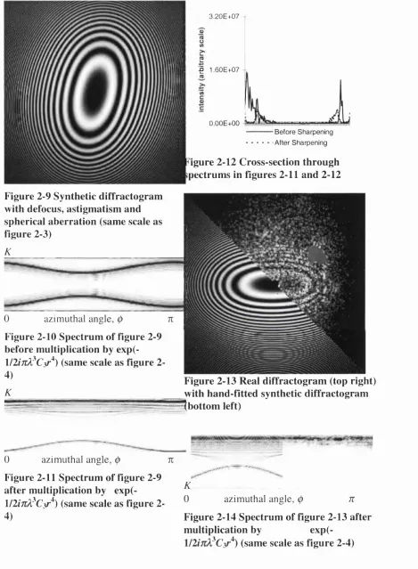
Figure 6-4 Dijfractogram fit. The top right-hand h a lf shows the original image; the bottom h a lf shows a

hand-fitted theoretical dijfractogram ____________________________________________________________________________________________________127

Figure 6-5 Block diagram o f the lens aberration determination system_______________________________________________131

Figure 6 - 6 Parameter interaction with the correlator m odule.______________________________________________________________133

Figure 6-7 Correlation score C( (j)) versus rotation angle (f) o f dijfractogram before folding._______________134

Figure 6 - 8 The three-component model o f the synthetic dijfractogram pattern.___________________________________136

Figure 6-9 Predicted ratio o f correlation value at peak (Cpeak) to mean correlation value away fro m peak

or minima (Cmean). __________________________________________________________________________________________________________________________________141

Figure 6-10 Predicted ratio o f the mean correlation value away fro m peaks or minima (Cmean) to the

expected correlation value at the minima (Cmin).____________________________________________________________________________________141

Figure 6-11 By fitting a quadratic curve to the minimum o f the correlation junction, an approximate

estimate o f the apparent prim ary astigmatism coefficient A j can be obtained using eq(6-44)._____________146

Figure 6-12 Illustration o f the effect o f noise in uncertainty in the correlation minima p o sitio n ._______149

Figure 6-13 The param eter interaction with the correlator and minimum m o d u le._____________________________151

Figure 6-14 Actual correlation minimum fo r the dijfractogram shown in Figure 6 -4 ._________________________157

Figure 6-15 Cross section through the minimum shown in Figure 6 - 1 4 .______________________________________________158

Figure 6-16 Contour p lo t o f the correlation function C(A],Cj) over a wide range o f A] and C j._________158

Figure 6-17 Variation in enclosed energy as a function o f the radius o f integration. _________________________160

Figure 7-1 Bin layout in UO3 storage facility. ______________________________________________________________________________________175

Figure 7-2 SG V with test dru m s.____________________________________________________________________________________________________________177

Figure 7-3 UO3 D rum s.__________________________________________________________________________________________________________________________177

Figure 7-4 A block diagram o f the image processing s y s te m________________________________________________________________178

Figure 7-5 Simplified block diagram o f the image processing system __________________________________________________180

Figure 7-6 Parameter propagation fo r the drum location system__________________________________________________________181

Figure 7-7 Interaction o f param eters with the thresholder m o d u le.______________________________________________________183

Figure 7-8 The effect o f noise on the probability o f a pixel being above the threshold._______________________184

Figure 7-9 Interaction o f param eters with the linker module. ______________________________________________________________187

Figure 7-10 Graph showing the probability o f a pixel having a grey-level above the threshold, in the

region where the illumination gradient intersects the threshold. __________________________________________________________188

Figure 7-12 Probability function o f a pixel being above the threshold, l-m (x,y) (dotted line) and

corresponding probability o f being linked, p(x,y) (continuous line). ____________________________________________________189

Figure 7-13 Parameter interactions fo r the centroid finding algorithm________________________________________________191

Figure 7-14 Original Image __________________________________________________________________________________________________________________195

(14)

Figure 7-16 Above image after linking. The non-connected pixels have been removed. _____________________195

Figure 7-17 Illumination surface____________________________________________________________________________________________________________195

Figure 7-18 Predicted values ofm (x,y)+ n(x,y) corresponding to the threholded im a g e._____________________195

Figure 7-19 Predicted values ofp(x,y)+q(x,y), scaled as above. __________________________________________________________195

Figure 7-20 Graph o f the actual positioning error (continuous line) and predicted positioning error

(broken line) in locating the drum cap as a function o f the uncertainty in apparent cap size, A min/A. 196

Figure A - l Error correcting Bullseye code used in chapter 5 .______________________________________________________________209

Figure B -l An example o f a specimen taken fro m an ovarian tum our.__________________________________________________211

Figure B-2 Voronoi diagram generated fro m cell nuclei (from [ 1 0 3 ] )._______________________________________________212

Figure B-3 Quadratic boundary fit to a segmented region o f epithelium (from [1 0 3 ])._______________________213

Figure B-4 Diagram showing complete information streams and perform ance parameters fo r the ovarian

cancer detection system. ________________________________________________________________________________________________________________________215

Figure B-5 Typical image fro m the intruder detection system showing an intruder (centre) entering the

sterile zone between the two fences. [Image courtesy o fP S D B ]____________________________________________________________217

(15)

List of Tables

Table 4-1 The parameters affecting the performance o f the ladle tracking algorithm...73

Table 5-1 Relative ranking o f phenomena which might affect the performance o f the proposed image processing system...8 8 Table 5-2 M odelling the parameters which affect the performance o f the system, and the variables used to describe them...91

Table 5-3 Comparison o f the parameters fo r the various code d esig n s...112

Table 5-4 Estimates o f param eter values fo r the operating conditions in the steelw orks...114

Table 6-1 Parameters affecting the performance o f the lens aberration determination system...129

Table 7-1 Parameters affecting the performance o f the IP system on the SG V...177

Table 7-2 The param eters describing the f i t fo r each o f the 12 illumination conditions tested....190

Table A -l Length, n, number o f information bits, k, and distance, d o f some optimum codes [78]...206

Table B -l Statistics generated by the boundary detection algorithm (from [1 0 3 ]):...213

Table B-2 Parameters affecting the performance o f the ovarian cancer detection system...214

(16)

Chapter 1:

Introduction

The field of image processing (IP) systems currently lacks a formalised structure, or methodology, for developing and assessing the performance of such systems. This often leads to a somewhat ad hoc approach to development, with systems being built and then tested, without their likely performance being calculated beforehand. This thesis describes a novel methodology which has been developed to assist engineers in both the development of IP systems and the prediction and characterisation of their performance.

1.1 Motivation - The Need for Performance Data

One of the key issues for engineers working in the development of IP and computer vision as an engineering discipline, is the relative lack of work being done to measure the performance of image processing algorithms and systems, and the consequent lack of data. For the engineers involved, this makes the design of systems far harder [1 ,2 ] and diagnostics more difficult [3]. This often results in a less systematic approach to development and testing, with less reliable systems being built. In turn, IP sometimes suffers from a problem of being seen as something of an immature technology and may consequently be underused. Producing a way to measure system performance or reliability will have the following main benefits:

Aiding Algorithm Development

By enabling researchers to measure the performance of their algorithm relative to existing techniques, a developer can quantify any improvements that each alteration causes and can more readily arrive at a better solution. He or she can also compare the effects of combining different algorithm components and using different values for tuning parameters.

Predicting System Suitability

If a system performance for a given task can be predicted from previously acquired data, its suitability for the task can be evaluated and testing and development time reduced.

(17)

Knowledge of the performance of different algorithms can aid the selection of the most appropriate technique for a given problem.

System Optimisation

If an envelope describing the performance of a system can be created, then this can be used as part of the input to a system optimisation technique. This will ultimately enable the optimum operating point for a system to be determined given the constraints of the task.

It is thus imperative that image processing starts to develop the sort of tools and information for performance measurement that are taken for granted in other disciplines of engineering.

1.2 Developing Performance Prediction Techniques

Predicting and characterising the performance of IP systems is difficult, mainly for the following reasons (some from [4]):

• Performance evaluation is task dependent. The overall system performance is a function of both the effectiveness of the algorithm, and the conditions under which it is operating. It is usually necessary to decouple these two factors. This enables the performance of a given system to continue to be predicted even when the operating conditions change, and brings universal performance measurement a step closer. • Different tasks require different performance measures. The metrics used to

characterise the performance of a tracking algorithm will differ from those which are used to measure the performance of an optical character recognition algorithm, and must be selected appropriately.

• The operating conditions must be characterised. Describing complex imaging conditions quantitatively is difficult.

• Vision is often only one component of a larger system. Other non-imaging factors may affect the overall performance, which must be taken into account.

• Vision is complex. The vision system often consists of several component algorithms which are combined to solve a vision task.

(18)

• Different performance measures mean that different systems cannot be compared directly.

• Algorithms are often developed without an accompanying theory, which makes their performance difficult to analyse.

• Algorithms often have many tuning parameters which may critically affect system performance. Any characterisation must also take these into account.

• Ground truth is expensive to acquire and is always open to interpretation. Just because a human operator indicates the position of a target does not mean it is the true position.

• Testing is time-consuming and is often not recognised as valuable research, particularly in academic publications. For example, in a recent conference (ICPR ’98), only six papers out of 494 directly addressed performance assessment issues. Most of the remainder presented new algorithms or techniques, and only a quarter of these provided any comparisons with existing algorithms. Less than a fifth analysed performance in a quantitative fashion beyond this.

These factors combine to make the task of IP system performance characterisation a challenging but important area of research.

1.3 Scope of this Research

This thesis goes some way towards addressing some of the deficiencies in IP system development and attempts to overcome some of the main difficulties in performance characterisation that have been outlined above. It contains a new methodology or ‘rule book’, which is intended to assist engineers and researchers in developing IP systems and algorithms. Although techniques have been developed for assessing individual algorithms, e.g. edge detection, segmentation etc., the author believes that no one has to date developed a generalised methodology for IP performance assessment for the system user. This new methodology will:

• Enable the analysis and performance predictions for a wide range of IP systems, even when they are applied to a variety of problems.

(19)

• Guide developers in analysing EP problems, decoupling the system from the operating conditions, gathering the appropriate data, then categorising the problem according to a set of criteria developed here.

• Describe a new technique for modularising IP systems, and for considering the system as a series of boxes, which propagate performance or quality characteristics in addition to data.

• Show how the interaction between the different modules and the parameters can be analysed.

• Demonstrate how the analysis of each of these modules can then be considered as a relatively simple transfer function between operating conditions and the module performance.

• Guide the developer in how to combine these transfer functions to derive overall performance estimates for a system under different operating conditions.

• Provide the building blocks for universal performance data predictors that can accompany off-the-shelf algorithms.

• Supply the necessary performance data which could then be used to optimise system performance.

The thesis demonstrates the effectiveness of the new methodology with a detailed assessment of four real-life IP problems, and a demonstration of how it could be applied to a further two problems. These show how the methodology can be used to analyse a variety of IP tasks, and how in practice it achieves the goals set out above.

1.4 Structure of this Thesis

The remainder of this thesis, consisting of eight chapters, is structured as follows:

(20)

Chapter 3 describes the new methodology in depth. It describes the steps which an IP system developer should take when developing and evaluating a system. This forms the structure of chapters 4-8, which apply the methodology to the performance analysis of real-world industrial IP problems.

Chapter 4 contains the performance analysis of the first of the IP applications. It uses a semi-empirical approach to evaluating an existing algorithm for use in tracking ladles of molten steel in a steelworks. It gives estimates of the likely final performance of a vision system used to solve this problem, and shows how the problem may not be amenable to an IP solution.

Chapter 5 is a mainly theoretical performance analysis of a second IP system for use in a steelworks, for identifying batches of steel. It includes a new error-correcting code developed by the author for this application.

Chapter 6 analyses the performance of a system for determining the aberrations in transmission electron microscope (TEM) lenses. It describes a new theoretical model of the image and the algorithm for calculating the errors in the estimates of the aberrations. The theoretical model was developed in collaboration with the author's supervisor, the application of the methodology is the authors work alone.

Chapter 7 analyses the performance of a vision system which is currently in operation on a self-guided vehicle manoeuvring drums of nuclear waste around a storage plant.

Chapter 9 concludes the thesis with a discussion of the research and suggestions for further research.

(21)

(22)

Chapter 2:

Background

This chapter describes the current state of the art in measuring the performance of image processing systems, and outlines the different approaches that have been adopted. It shows where this thesis fits into current research, insofar as it represents the first attempt at a complete methodology for performance characterisation. The work described in this thesis is intended for image processing system developers who are interested in evaluating the performance of systems they design. The chapter finishes by describing some of the image processing techniques which will be used later in the thesis.

2.1 Performance Measurement in other Engineering Disciplines

Performance measurement in other engineering disciplines is highly developed. An engineer will choose the best specified product for a task, as it can often be determined without testing whether the product is a suitable candidate for the task in hand. This choice is often achieved using the following techniques:

1. Standardisation

Using standard fittings, sizes, interfaces etc., in order to avoid compatibility problems.

2. Modularisation

Breaking the system down into smaller functional blocks allows the performance of these blocks to be analysed individually and then combined to predict the performance of the system as a whole.

3. Theoretical Models

The performance of many engineering systems is evaluated using theoretical expressions describing the behaviour of materials, fluids, components etc. and can be evaluated by hand or numerically by computer.

(23)

variety of conditions. These may be taken from tests of the actual devices operating in situ, or from scale models, simulations in wind tunnels etc.

In the field of image processing, the first technique is being tackled by IP researchers [5] and is not being addressed in this thesis. However techniques 2, 3 and 4 are often taught to engineers during training. In some disciplines, such as computer aided engineering, these procedures are formalised further, by the development of methodologies for specifying, designing and breaking down engineering problems [6-9]. There have also been similar tools developed for assessing the performance of computer code [10]. The techniques of modularisation, theoretical modelling and testing inspired much of the methodology development that is described in the remainder of the thesis.

2.2 Different Techniques for Measuring Performance

Three main techniques for measuring performance of image processing algorithms and systems have begun to be developed. These are performance characterisation, performance evaluation and benchmarking. This section describes the differences between them and how work in each field has developed so far.

2.2.1 P erfo rm an ce Characterisation

Performance characterisation is usually defined in IP to mean the measurement or prediction of the performance of an algorithm or system throughout the full space of the expected operating conditions. This performance characterisation, although time- consuming, can then be used to predict performance when a system is used for a new application or under different imaging conditions. Different methods for performance characterisation, such as testing and analytical algorithmic modelling have been developed, and are described in sections 2.2.1.1 to 2.2.1.3.

(24)

segmentation [15, 16], image stabilisation [17], and algorithms such as pixel vectorisation [18], binarisation [19], and detection algorithms [20].

2.2.1.1 Algorithmic Modelling

A formal description of algorithmic modelling was given in [21] as a way of characterising algorithm performance. Algorithms are developed in conjunction with a mathematical (analytical) model of the algorithm that describes their performance. This model can then be used as a transfer function, to calculate performance, given the input operating conditions. For example, analytic models of line and circle fitting algorithms have been developed, which enable the estimation of errors when input variables such as line length and noise are varied. These predictions are then compared with results from empirical tests on synthetic data [22]. Other models have been used to estimate various location and detection errors in com er detection algorithms as noise levels vary [23].

One of the most important features of algorithmic modelling, which is not addressed in the literature but forms an important part of this thesis, is parameter determination. The effectiveness of the algorithm model depends critically upon selecting the appropriate parameters to describe the input conditions and performance metrics. Selection of parameters is discussed in chapter 3.

(25)

2.2.1.2 Perform ance Envelope M easurem ent

The performance envelope specifies the performance of a system as the parameters describing the operating conditions are varied. It is a surface in a multidimensional space, with each dimension corresponding to an input parameter or performance metric. A simple one-dimensional example is the speed/altitude capability of an aircraft. The performance envelope can either be calculated using the algorithmic modelling method described in section 2.2.1.1, or be measured by using the testing techniques discussed in section 2.2.1.3. Either method requires appropriate parameter selection to ensure the dimensions in the space correspond with the most important measures of the input conditions.

Once calculated, either theoretically or empirically, the performance envelope can then be used to determine the performance of a system under known operating conditions.

2.2.1.3 Testing

One method of evaluating performance is simply to implement the system and test it on real data. As this thesis will show, under some conditions this may be necessary. Haralick [24] proposed that both performance evaluation and characterisation can be carried out by describing the ‘normal’ operating conditions (i.e. input data), then randomly perturbing the operating position and measuring the effect on performance. However the probability distribution of the actual operating conditions is critical to overall system performance, and must be taken into account.

(26)

conditions, than with the algorithm itself. A discussion of the use of testing for performance characterisation is given in [25].

2.2.2 Perform ance Evaluation

Performance evaluation differs from performance characterisation in that it is only trying to measure performance against a pass/fail criterion. This means that for a given algorithm, only a subspace of possible operating condition needs to be analysed, namely those conditions under which the algorithm will be operating under when performing the task for which it is being considered. It also means that certain performance characteristics, which it would be necessary to measure for complete characterisation, can now be neglected. The advantage of performance evaluation over characterisation is therefore ease of implementation. However it does not give a complete description of system performance and therefore is not valid if the operating conditions change or if the system is used for a different task.

2.2.3 Benchmarking

Benchmarking differs substantially from the previous two techniques. Benchmarking implies a common, ‘level playing-field’ test, whereby an identical task is carried out with a variety of algorithms and each is given a performance measure. A familiar example from outside the field of IP is the DOT fuel consumption test, where every vehicle is tested for fuel consumption under a specified set of driving conditions and given a figure of performance.

2.2.3.1 Exam ples of Benchmarking

(27)

aims and achievements were to compare the parallel computers on which the algorithms were run, rather than to compare the algorithms themselves.

2 .2 .3 .2 The “StatLog” Project

The ESPRIT-funded StatLog project, which ran from 1990-1993, was designed to provide a quantitative comparison of a wide range of classification algorithms, by testing their relative performance under ‘level playing field’ conditions against a wide range of classification tasks, although only a few of these used image databases. The classification algorithms fell into three main categories - statistics-based, machine learning based, and neural networks. The results of this project are summarised in a book on the project [34].

Statistics-based algorithms are generally considered to have an explicit underlying probability model, and it is usually assumed that the algorithms can be ‘tuned’ by humans (mainly statisticians), who can control the overall flow of the algorithm. Machine learning (ML) is based on earlier artificial intelligence ideas, which usually try to construct decision trees ( ‘if-then’ rules) based on the supplied training data. The term ‘neural networks’ covers a wide range of algorithms, but is usually taken to imply a network of one or more interconnected layers of nodes ( ‘neurons’) which are trained to adjust their contents in response to repetitive presentation of a set of training patterns. The training may be supervised or unsupervised. Supervised learning, requires the user to input the class of each training pattern. Unsupervised learning extracts information about the training data set without explicit guidance during training, but the user has subsequently to specify which system response corresponds to which category.

The StatLog project provided an excellent review of these different approaches and provides a role model for any benchmarking studies, whether in the field of image processing or in other areas where classification is needed.

(28)

under which the system will be used, the results will be inaccurate as a predictor of system performance. However benchmarking does allow a direct comparison between algorithms. Developers often find this idea attractive as they want to know which algorithm is the ‘best’. Unfortunately performance depends critically on the operating conditions, so that without a very careful choice of tests, such comparisons can be misleading.

Therefore for the reasons described above, benchmarking will not be considered further in the remainder of this thesis.

2.2.4 M odularisation

The modularisation of algorithms has been suggested as an aid to performance characterisation [4, 35, 36J. Breaking down the algorithm allows individual sections to be analysed. These less complex sub-systems can then be analysed, and their performance characteristics combined with those of the other modules to yield a final performance measure. One of the most important aspects of modularisation is the use of quality metrics, which determine how the performance characteristics of each module are propagated through the system. This is described briefly in [35], and is developed in more depth in chapter 3.

Modularisation greatly facilitates the analysis of IP system performance. Algorithm modules are usually less complex than the system as a whole, and are consequently easier to model. Modularisation also enables different sub-system algorithms to be included in the overall system, and the performance analysis can be updated readily to measure the affects of the change. Methods for system modularisation are developed in chapter 3, and demonstrated extensively in chapters 4-8.

2.3 Related Work

(29)

2.3.1 S tandarisation

Attempts to impose standards in image processing have followed two main lines of development: standardising the frameworks for development and testing and standardising databases of test images.

2.3.2 S tan d ard Fram ew orks

2.3.2.1 Im age U nderstanding Environment (IUE)

The IUE is a five-year US program, sponsored by the Defence Advanced Research Projects Agency (DARPA), to develop a common software environment for the development of algorithms and application systems [5]. Its goals are to improve research productivity, to provide a standardised format for education and development, to standardise computational models and to improve technology transfer. It can be used as a basis for algorithm development. DARPA had earlier produced a ‘DARPA benchmark’ - a set of test images (of moving, overlapping rectangles) which was used as a test piece for comparing the relative performance of various algorithms.

2.3.2.2 Im age P rocessing S tandards/B SI Collaboration

The standards organisations ISO and IEC set up a joint technical committee to investigate the possible provision of standards for image processing. A working group (ISO/IEC JTC 1/SC 24/WG7) failed to reach a consensus on the correct approach to take.

2.3.2.3 H arn ess for Algorithmic Testing and Evaluation (HATE)

(30)

2.3.2.4 S tandard Image D a tab ases

A different approach to comparing algorithm performance is to provide databases of standard images, covering a wide range of operating conditions against which algorithms can be tested. Several of these exist, such as the National Institute of Standards in Technology (NIST) database of handwritten zip codes, British Aerospace’s segmentation databases [37] and many more are being developed. Examples include databases for face recognition tasks [38], automated manufacturing [39] and more general image databases [40].

2.3.2.5 Automatic Algorithm Tuning

Automatic selection of algorithm tuning parameters and automatic system configuration is an area in which some related work has been carried out. Any optimising technique requires a ‘fitness’ measure, which in turn implies performance meaurement. This development has yielded some novel ways of performance measurement. For example, Ramesh and Haralick [41] describe a methodology to optimise the selection of algorithm tuning parameters, by minimising appropriate performance measures. They demonstrate the technique on an algorithm for edge detection and linking. Similar techniques have been developed in other area of IP such as boundary detection [42], automatic target recognition [43] and the selection of edge detection algorithms [44].

2.3.2.6 Statistical T echniques for Algorithm Testing

(31)

modelling errors [54]. Also important is the effect of different non-linear functions on the propagation of variance [55].

2.3.2.7 Real-World Algorithm Developm ent and Testing

Some of the more useful research work in performance evaluation has stemmed from attempts by designers to characterise the performance of real-world systems as they are developed. These have the advantage of addressing the complexity often present in real-world IP problems [56-59] [43]. Some have considered the different modular stages in an algorithm [60], though have not attempted to analyse their performance in-depth.

Im age Characterisation and Perform ance Metrics

An important feature of any characterisation or evaluation procedure is the necessity to measure the appropriate characteristics of the input data. This has been attempted for several types of algorithm and problem [61-63]. There have also been attempts to develop appropriate performance metrics for different IP tasks such as image segmentation [13, 37, 64], and also in related fields such as non-destructive testing, where the probability of detection (POD) is used to measure performance as a function of defect size [65]. One of the most useful measures developed is the receiver operating characteristic (ROC) curve. This plots the probability of false indications (PFI) against the POD as a function of some classification threshold [6 6]. Although this yields a curve in two-dimensions, it can be turned into a useful one-dimensional performance measure by integrating the area under the curve [67].

2.4 Background on Techniques

(32)

describes some of the different techniques which have been developed in an attempt to determine the lens aberrations in transmission electron microscopes (TEMs), the problem analysed in chapter 6. There is then an introduction to the theory of error- correcting codes, which are used in chapter 5 in ladle identification. Different algorithms that could have been used in chapter 7 on drum location are not described here, as the algorithm had already been designed by the plant operators. Their system design is described in chapter 7.

2.4.1 T em plate Matching

Template matching based on correlation is used for determining whether and where a specific reference pattern (the template) is located within an input image (the scene). It is typically used for detecting and locating objects of known sizes and orientations in scenes.

If t(i,j) refers to the pixel grey level at position (ij) in the M x N template image and s(i-m,j-n) refers to the corresponding grey level in the scene image when the template is displaced by some distance (m,n). The difference correlation measure or

score at position (m,n) is then calculated according to [6 8]:

m + M - ln + N - l 2

D(m, n)= X X \t(i, j) - s{i - m , j - n)\ i=m j=n

eq(2-l) Expanding this yields the form:

D(m, n) = X X |t(i, j)\2 + X X |s(i, j ) f - 2 X X t{i, j)s{i - m , j - n) i-m j - n i-m j=n i=m j=n

(33)

m + M - l n + N - \ ~

2 2 - » i , j - « ) |

D(m,n) = i=m i=n ---/ z s K i j f z s I s M 2 V 1 J * J

eq(2-3) or the normalised cross correlation coefficient:

C{m,n) =

m + M - ln + N - l

X ' L t ( i , j ) s ( i - m , j - n ) i=m j=n

J z 2 H U ) | 2 Z 2 k < J ) |2

V * 7 *' j

eq(2-4) The Cauchy-Schwarz inequality states that:

X X t( i , j ) s ( i - m , j - n) i j

eq(2-5) Equality holds i f and only if:

t ( i , j ) = a r ( i - m , j - n ) , i = m,....,m + M — 1 j = n ,....,n +N - I

eq(2-6) where a is a constant. Hence c(m,n) is always less than or equal to unity and reaches a maximum value of unity if the template is an exact, replica of the scene at (m,n). A variety of templates enables this technique to be used to search not only for the location of an object, but also to identify the size and type of object visible in the image.

2.4.2 Tracking

(34)

The linear Kalman filter is a classic tool of optimal estimation theory [69]. It is based on a model of a physical system involving a time dependent state vector, x, and a set of linear equations called the system model. The state vector contains enough variables to describe the dynamic properties of a system. In the case of tracking an object in three dimensions, velocity and displacement in each direction are sufficient. The system model describes the change in state over time. If we sample at equally spaced time periods, tk=to+kAT, with k = 0,1, ... and A T a sampling interval. The linear system can be modelled in vector form

Xk = Ok-iXk-i + £k-i

eq(2-7) where £k_i is a vector indicating random additive noise. The state transition vector Ok-i is also a function of time to allow for complex system dynamics. A noisy measurement is made of the state vector at time tk and the Kalman filter theory assumes that the following relation holds:

Zk = 7/kXk + Pk

eq(2-8) where Zk is the vector of measurements taken, is the measurement matrix and Pk a random vector modelling additive noise.

If pk and £k are white, zero-mean, Gaussian processes with covariance matrices

Qk and Rk the Kalman filter can be shown to be the optimal estimate of the state of the system [69].

The Kalman filter is implemented by evaluating the following recursive equations:

P k = 3>k-l Pk - l ^ k - l + Qk-l

(35)

x'k= Ok-ix'k-i + Kk(zk- HkOk.ix'k.i)

P k = ( I - K y ) P \ { I - K y f + K k R k K kT

eq(2-9,10,11,12) where x'k is the optimal state estimate at time rk- Pk is the a priori estimate of the error covariance and is the gain or blending factor that minimises the a posteriori error covariance.

If x is a 2-D state vector [jci,X2]T, the region of the plane centred around x'k which contains the true state with a given probability c2 is the ellipse

(x - x'kX Pk)~\x - x'k)T < c2

eq(2-13) The axes of this ellipse are ±cV^ei, i = 1,2, where Xj and e* are the eigenvalues and eigenvectors, respectively, of Pk- This uncertainty ellipse can then be used to calculate the search space for the next frame in the tracking sequence.

For the example tracking problem discussed in chapter 4 however, the time dependency of ^>k is not known, due to the sudden changes in acceleration of the object. Ok could model the inertia of the object being tracked, i.e. assuming no acceleration, which would provide a good estimate of state during relative simple motion. However changes in acceleration are frequent enough in this application that the improvement in system performance is likely to be secondary to other factors. For this reason, and to simplify some of the analysis, the use of a Kalman filter is not considered in chapter 4.

(36)

and some of the other techniques for lens aberration determination which have been described in the literature are discussed.

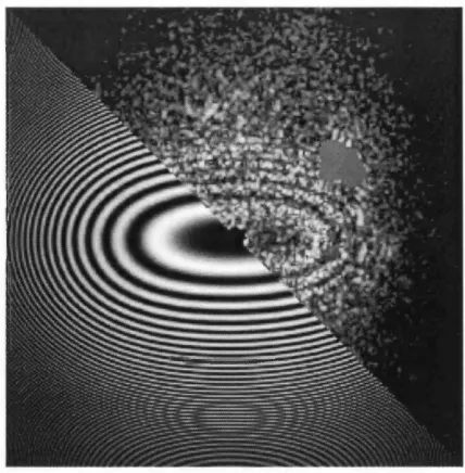
The TEM can be used to generate a diffractogram, see Figure 2-1, the intensity of which describes a function of the form (from [73]).

F (r, 0 ) = sin2 0rA3 C3 r4 / 2 - ttAC, r2 / r2 / 2) cos(2(0 - 0 22)))

eq(2-14) The reasons for the function having this form are explained in chapter 6.

The image processing problem is to fit this function to the noisy data in the diffractogram and hence deduce the values of the parameters for the spherical aberration, C3; defocus, C\, two-fold astigmatism, A\, and the angle of primary astigmatism, 022- (The actual aberration determination procedure is more complex, as other aberrations exist which must be measured by producing images with an induced tilt in the electron beam. This is discussed in chapter 6.)

2.4.3.1 M anual Fitting

(37)

Figure 2-1 A d iffracto g ram from a transm ission electron microscope. The to p -rig h t of the im age shows the original d iffracto g ram , the bottom left a synthetic d iffracto g ram w hich has been m anually fitted to the data.

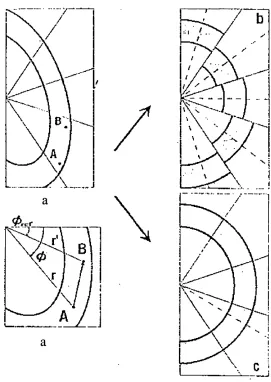
2.4.3.2 Stretch R em apping

One possible automated solution is to integrate the signal strength tangentially

around the diffractogram. This improves the signal to noise ratio and can be achieved

quite easily when the diffractogram is circular, i.e. when the astigmatism is small.

However when astigmatism is significant, other techniques must be employed. One such

method is sector averaging, as proposed in [73]. This involves assuming that the

diffractogram is approximately circularly symmetrical over a small angle and integrating

tangentially through this angle (an angle of 36° was chosen for this particular

diffractogram as an optimal compromise between maximising the number of data points

used for the integral and minimising the variation in the diffractogram over the sector.

Where fewer rings are visible in the diffractogram, the size of the angle has to be

increased to e.g. 60°, to get acceptable errors [73]). The result can be used to find an

approximation to the position of the zeroes in the function. This information can then be

fed back to ‘stretch’ the diffractogram to approximately circularly symmetrical, as

(38)

a

/ b

/

Figure 2-2 Use of ‘sector averaging’ technique to perform tangential integration on non-circular diffractograms. (from [73])

From the original image a, an approximation of the radius r over sector (j) is made. The radius is then scaled to convert the image, assumed to approximate image b, into a circularly symmetrical diffractogram as shown in c. Although this overcomes some of the problems due to noise, it seems rather crude and error prone to approximate some of the sectors as circular.

2.4.3.3 Rem apping and Fourier Analysis

(39)

of the spherical aberration, C3, to within a reasonable degree of accuracy. The principal

behind the approach is that

sin2( y ) - — = exp(i7rACjr2)expf—i^A3C3r4 - —exp(- /7rAC1r2)e x p f- — inX3C3r.4

eq(2-15) M ultiplication by

e x p (- 1/2 z7rA3 C3r 4)

and substitution of K = r 2 gives

eq(2-16)

sin 2(y ) = i - -^-exp (/TrAC1! AT)- —e x p ( - i n X C xr K )exp ( - inA,3C3K )

eq(2-17) Taking the Fourier Transform of this function with respect to AT, the spatial frequency squared, should yield peaks at Af=±l/27rACi. Thus C\ can be determined if the position of the peaks can be found and measured.

This works well on synthetic data, as shown below. It requires good estimates of the background, as this should be subtracted from the image to minimise the effect of low frequency components obscuring the true signal peak.

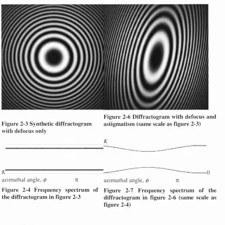
Figure 2-3 shows a noise-free synthetic diffractogram with defocus, C1, the only aberration. Figure 2-4 is the spectrum with K on the vertical axis and azimuthal angle, (j),

along the horizontal axis. Spherical aberration, C3, is zero, so the e x p (-l/2/7rA3C3r4) term

is unity. As expected, the image gives two sharp lines at ^T=±1/2tiACi. There is no (j)

dependency due to the circular symmetry of the diffractogram. Figure 2-5 is a cross- section through Figure 2-4, clearly showing the two peaks.

(40)

Figure 2-9 to Figure 2-12 demonstrate the effects of the inclusion of spherical aberration. Figure 2-9 is a diffractogram generated with a spherical aberration term. Figure 2-10 is the spectrum without multiplying by the ex p (-l/2/7rA3C3r4) term. It can be seen that the K2 term due to the spherical aberration has blurred the peaks. Figure 2-11 shows the spectrum after multiplication by ex p (-l/2z7rA3C3r4). One of the peaks (the lower sinusoid) is sharpened; the other is blurred completely.

(41)

Figure 2-6 D iffractogram w ith defocus and Figure 2-3 Synthetic d iffracto g ram astigm atism (same scale as figure 2-3) with defocus only