Scholarship@Western
Scholarship@Western
Electronic Thesis and Dissertation Repository
7-31-2012 12:00 AM
Further applications of higher-order Markov chains and
Further applications of higher-order Markov chains and
developments in regime-switching models
developments in regime-switching models
Xiaojing Xi
The University of Western Ontario
Supervisor Rogemar Mamon
The University of Western Ontario
Graduate Program in Applied Mathematics
A thesis submitted in partial fulfillment of the requirements for the degree in Doctor of Philosophy
© Xiaojing Xi 2012
Follow this and additional works at: https://ir.lib.uwo.ca/etd Part of the Other Applied Mathematics Commons
Recommended Citation Recommended Citation
Xi, Xiaojing, "Further applications of higher-order Markov chains and developments in regime-switching models" (2012). Electronic Thesis and Dissertation Repository. 678.
https://ir.lib.uwo.ca/etd/678
This Dissertation/Thesis is brought to you for free and open access by Scholarship@Western. It has been accepted for inclusion in Electronic Thesis and Dissertation Repository by an authorized administrator of
CHAINS AND DEVELOPMENTS IN REGIME-SWITCHING
MODELS
(Spine title: Higher-order Markov chains and regime-switching models)
(Thesis format: Integrated Article)
by
Xiaojing Xi
Graduate Program in Applied Mathematics
A thesis submitted in partial fulfillment
of the requirements for the degree of
Doctor of Philosophy
The School of Graduate and Postdoctoral Studies
The University of Western Ontario
London, Ontario, Canada
c
CERTIFICATE OF EXAMINATION
Supervisor:
Dr. Rogemar Mamon
Co-Supervisor:
Dr. Marianito Rodrigo
Examiners:
Dr. Adam Metzler
Dr. Mark Reesor
Dr. Hao Yu
Dr. Anatoliy Swishchuk
The thesis by
Xiaojing Xi
entitled:
Further applications of higher-order Markov chains and developments in regime-switching models
is accepted in partial fulfillment of the requirements for the degree of
Doctor of Philosophy
Date Chair of the Thesis Examination Board
We consider higher-order hidden Markov models (HMM), also called weak HMM (WHMM),
to capture the regime-switching and memory properties of financial time series. A technique of
transforming a WHMM into a regular HMM is employed, which in turn enables the
develop-ment of recursive filters. With the use of the change of reference probability measure
method-ology and EM algorithm, a dynamic estimation of model parameters is obtained. Several
applications and extensions were investigated. WHMM is adopted in describing the evolution
of asset prices and its performance is examined through a forecasting analysis. This is
ex-tended to the case when the drift and volatility components of the logreturns are modulated by
two independent WHMMs that do not necessarily have the same number of states. Numerical
experiment is conducted based on simulated data to demonstrate the ability of our estimation
approach in recovering the “true” model parameters. The analogue of recursive filtering and
parameter estimation to handle multivariate data is also established. Some aspects of
statisti-cal inference arising from model implementation such as the assessment of model adequacy
and goodness of fit are examined and addressed. The usefulness of the WHMM framework
is tested on an asset allocation problem whereby investors determine the optimal investment
strategy for the next time step through the results of the algorithm procedure. As an application
in the modeling of yield curves, it is shown that the WHMM, with its memory-capturing
mech-anism, outperforms the usual HMM. A mean-reverting interest rate model is further developed
whereby its parameters are modulated by a WHMM along with the formulation of a self-tuning
parameter estimation. Finally, we propose an inverse Stieltjes moment approach to solve the
inverse problem of calibration inherent in an HMM-based regime-switching set-up.
Keywords: Higher-order Markov chain, filtering, change of reference probability method,
asset price modeling, forecasting, asset allocation, multivariate data, term structure of interest
rates, inverse problem in finance
I hereby declare that this thesis incorporates materials that are direct results of several joint
research collaborations. My research outputs with my supervisor, Dr. Marianito Rodrigo
(co-supervisor) and Dr. Matt Davison have already led to published papers and manuscripts under
review in various peer-reviewed journals and refereed book chapters. These are detailed below.
The content of chapter 2 appeared as a published article (co-authored with my supervisor, Dr.
Rogemar Mamon) in the journal Economic Modelling; see reference [25] of chapter 3.
Chapter 3 is currently being converted into a manuscript (co-authored with Dr. Mamon) and
will be submitted for publication in the journal Systems and Control Letters.
Materials of chapter 4 are based on a manuscript (co-authored with Drs. Mamon and Davison)
that is presently under revision for the Journal of Mathematical Modelling and Algorithms.
This chapter already includes modifications to the original submission in an effort to address
comments and suggestions of two referees.
Chapter 5 is based on a manuscript (co-authored with Dr. Mamon) that was submitted (by
invi-tation) as a book chapter to a peer-reviewed monograph “State-Space Models and Applications
in Economics and Finance” edited by S. Wu and Y. Zeng and will be featured as part of the
new Springer Series Statistics and Econometrics for Finance.
Chapter 6 originated from a paper that is currently under review in the journal Statistics and
Computing.
The results of chapter 7 are contained in a paper that was already accepted in a refereed
monograph “Advances in Statistics, Probability and Actuarial Science” edited by S. Cohen,
As the first author of all the papers emanating from this research, I was in-charge of model
im-plementation, filtering algorithm developments, data collection and analysis, literature review
and completing the first draft of the manuscripts. With the exception of my supervisor and
co-supervisors guidance on modeling framework formulations, I certify that this dissertation is
fully a product of my own work.
I would like to sincerely thank all of the people who helped in the various stages of this
re-search. First and foremost, I would like to gratefully acknowledge my supervisor Dr. Rogemar
Mamon for his guidance and indispensable support in completing this research. I greatly
ad-mire him for his accessibility and patience, his professionalism and scientific insight. His
experience, suggestions and encouragement were priceless. I am also appreciative of the help
and support of my co-supervisor Dr. Marianito Rodrigo.
Sincere thanks are due to Dr. Matt Davison, Dr. Adam Metzler and Dr. Mark Reesor for
leading the Financial math group and providing a productive and fun research environment.
I wish to extend my warmest thanks to my course instructors Dr. Rob Corless and Dr. Greg
Reid. Their kind support and guidance have been of great value in this study. The
departmen-tal staff has also been tremendous; my sincere thanks to Audrey Kager and Karen Foullong
for answering all my questions and resolving issues of concern. I am grateful to my current
and former colleagues in the PhD program for making the dark, depressing hours seem brighter.
Finally my deepest gratitude goes to my family members, specially my parents for their
con-stant supports and encouragements throughout my life. I would like particularly to extend my
sincere gratitude to my loving husband for giving me strength during hard times. Without all
your loves, encouragements, and understanding it would never be possible for me to continue
my studies.
Certificate of Examination ii
Abstract iii
Co-Authorship Statement iv
Acknowledgments vi
List of Figures xii
List of Tables xiii
1 Introduction 1
1.1 Background and motivation . . . 1
1.2 Research objectives . . . 3
1.3 Literature . . . 4
1.4 Structure of the thesis . . . 5
References . . . 9
2 Parameter estimation of an asset price model driven by a WHMM 12 2.1 Introduction . . . 12
2.2 Description of a weak hidden Markov model . . . 15
2.3 Change of reference probability measure . . . 18
2.4 Calculation of recursive filters . . . 20
2.5 Parameter estimation . . . 23
2.7 Conclusion . . . 35
References . . . 37
3 Parameter estimation in a WHMM setting with independent drift and volatility components 40 3.1 Introduction . . . 40
3.2 Model background . . . 43
3.3 Filters and parameter estimation . . . 46
3.4 A simulation study . . . 52
3.5 Conclusion . . . 56
References . . . 57
4 A weak hidden Markov chain-modulated model for asset allocation 60 4.1 Introduction . . . 60
4.2 Filtering and parameter estimation . . . 66
4.3 Forecasting indices . . . 73
4.4 A switching investment strategy . . . 79
4.5 A mixed investment strategy . . . 83
4.6 Evaluating the portfolio performance . . . 86
4.7 Conclusion . . . 97
References . . . 99
5 Yield curve modeling using a multivariate higher-order HMM 103 5.1 Introduction . . . 103
5.2 Filtering and parameter estimation . . . 108
5.3 Implementation . . . 114
5.4 Forecasting and error analysis . . . 120
5.5 Conclusion . . . 125
6 An interest rate model incorporating memory and regime-switching 131
6.1 Introduction . . . 131
6.2 Model construction . . . 136
6.3 Filters and parameter estimation . . . 140
6.4 Implementation . . . 145
6.5 Forecasting and error analyses . . . 153
6.6 Conclusion . . . 160
References . . . 162
7 Parameter estimation of a regime-switching model 167 7.1 Introduction . . . 167
7.2 Regime-switching model setup . . . 170
7.3 Derivation of a system of Dupire-type PDEs . . . 173
7.4 Inverse Stieltjes moment problem . . . 175
7.5 Numerical implementation and results . . . 178
7.6 Implementation to “practical data” . . . 186
7.7 Conclusion . . . 192
References . . . 195
8 Concluding remarks 198 8.1 Summary and commentaries . . . 198
8.2 Further research directions . . . 200
References . . . 203
A Proof of equation(2.16) 204 B Proof of Proposition 2.4.1 205 B.1 Proof of equation (2.22) . . . 205
B.3 Proof of equation (2.24) . . . 207
C Proof of Proposition 2.5.1 208
C.1 Proof of equation (2.27) . . . 208
C.2 Proof of equation (2.28) . . . 209
C.3 Proof of equation (2.29) . . . 210
D Proof of Proposition 6.3.2 212
D.1 Proof of equation (6.25) . . . 212
D.2 Proof of equation (6.26) . . . 213
D.3 Proof of equation (6.27) . . . 214
E Proof of equation(6.36) 216
Curriculum Vitae 218
2.1 Evolution of estimates forf,σandA-matrix under the 2-state setting . . . 28
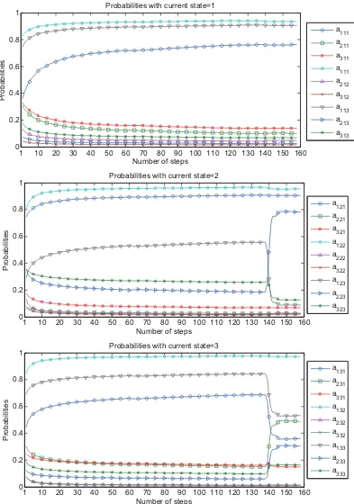
2.2 Evolution of estimates for the transition probabilities under the 3-state setting . 29
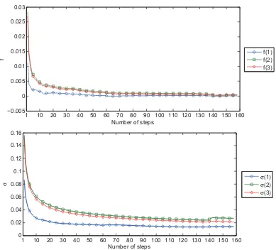
2.3 Evolution of estimates forfandσunder the 3-state setting . . . 30
3.1 Evolution of parameter estimates under different model settings . . . 55
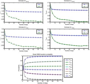
4.1 Evolution of parameter estimates under the 2-state setting . . . 76
4.2 Actual data and one-step ahead forecasts for Russell 3000 growth and value
indices (left), and zoom-in view for the period Jul 02 – Dec 05 (right) . . . 77
4.3 Actual returns and one-step ahead forecasts for returns of Russell 3000 growth
(left) and value (right) indices . . . 78
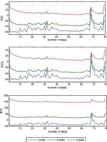
4.4 AIC, AICc and BIC values for the 1-, 2- and 3-state models . . . 80
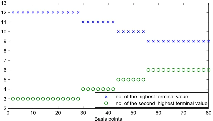
4.5 Numbers of the intervals switching strategy has the highest and the second
highest terminal values for varying transaction cost . . . 82
4.6 Optimal weights for Russell 3000 value and growth indices in the
WHMM-based mixed strategy withv= 0.08 . . . 85
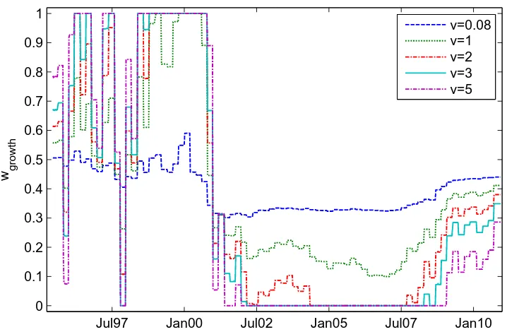
4.7 Evolution of optimal weights for Russell 3000 growth index in the
WHMM-based mixed strategy with varyingv’s . . . 85
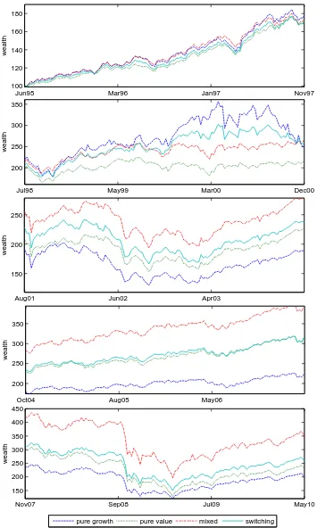
4.8 Switching, mixed, pure growth and pure value strategies comparison between
1995 and 2010 . . . 87
5.1 Evolution of estimates for transition probabilities through algorithm steps
un-der the 2-state setting . . . 117
5.3 Evolution of estimates forσthrough algorithm steps under the 2-state setting . 119
5.4 AIC for the 1-, 2-, 3- and 4-state models . . . 122
5.5 One-step ahead predicted values (%) versus actual Treasury yields (%) under a 2-state WHMM setting . . . 124
6.1 Evolution of estimates for transition probabilities under the 2-state setting . . . 148
6.2 Evolution of parameter estimates under the 2-state setting . . . 149
6.3 Evolution of parameter estimates under the 3-state setting . . . 151
6.4 Plot of actual and one-step ahead forecasts in a 2-state WHMM . . . 154
6.5 Plots of AIC values for 1-,2-,3- and 4-state WHMMs . . . 159
7.1 Actual and estimated call prices:λ1 =0.25,λ2 =2 andn= 2. . . 188
7.2 Actual and estimated call prices:λ=2 andn=7. . . 192
7.3 Actual and estimated call prices:λ1 =0.25,λ2 =1 andn=7. . . 194
2.1 Segregation of the period of actual data into two states . . . 26
2.2 Segregation of the period of actual data into three states . . . 26
2.3 Range of SEs for each parameter under the 1-, 2- and 3-state settings . . . 31
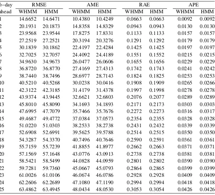
2.4 Error analysis of WHMM and HMM models under the 2-state setting . . . 33
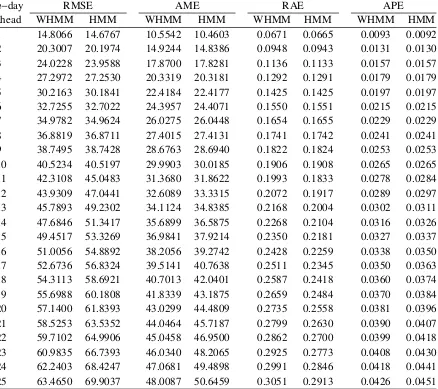
2.5 Error analysis of WHMM and HMM models under the 3-state setting . . . 34
3.1 Comparison of 1-step ahead forecast errors . . . 56
3.2 Comparison of 5-step ahead forecast errors . . . 56
4.1 Summary statistics of Russell 3000 growth returns . . . 74
4.2 Summary statistics of Russell 3000 value return . . . 74
4.3 Summary statistics of Russell 3000 return . . . 74
4.4 Error measures for one-step ahead forecasts under 1-, 2- and 3-state WHMM set-ups . . . 78
4.5 Performance comparison for WHMM- and HMM-based switching strategies with varying transaction costs. . . 82
4.6 Performance comparison between WHMM- and HMM-based mixed strategies with varying transaction costs. . . 86
4.7 Sharpe ratio for five investment strategies using 15 intervals. Numbers inside the parentheses are standard errors. . . 88
4.8 Jensen’s alpha for four investment strategies using 15 intervals. Numbers inside the parentheses are standard errors. . . 90
theses are standard errors. . . 91
4.10 p-values for the Jarque-Bera test of normality on data given in Tables 4.7 - 4.9 93 4.11 p-values for a one-tailed significance test on the performance results shown in Tables 4.8 - 4.9 . . . 93
4.12 p-values for a Wilcoxon rank sum test on the performance results shown in Tables 4.7 - 4.9 . . . 93
4.13 Performance evaluation for 10000 bootstrapped datasets with 5bps transaction cost . . . 95
4.14 Performance evaluation for 10000 bootstrapped datasets with 30bps transaction cost . . . 96
5.1 Descriptive summary statistics and data segregation into two states . . . 115
5.2 Segregation of data into three states . . . 115
5.3 Parameter estimates at the end of final algorithm step forN = 3 . . . 117
5.4 RMSE for one-step ahead predictions versus actual values . . . 122
5.5 Error analysis of WHMM and HMM models under the 1-state setting . . . 125
5.6 Error analysis of WHMM and HMM models under the 2-state setting . . . 125
5.7 Error analysis of WHMM and HMM models under the 3-state setting . . . 125
5.8 Error analysis of WHMM and HMM models under the 4-state setting . . . 126
6.1 Possible segregation of data into 2 states . . . 146
6.2 Possible segregation of data into 3 states . . . 146
6.3 Estimates ofHunder different estimators . . . 147
6.4 Range of SEs for each parameter under the 1-, 2-, 3- and 4-state settings . . . . 152
6.5 Error analysis for 2-state setting . . . 157
6.6 Error analysis for 3-state setting . . . 157
6.7 Error analysis for 4-state setting . . . 158
based on forecasting errors shown in Tables 6.5-6.7 . . . 158
6.9 p-values for a one-tailed significance test on the comparison of HMM and
WHMM based on forecasting errors shown in Tables 6.5-6.7 . . . 158
7.1 Example 1: Estimated parameters for different λ and n with σ1 = 0.1 and
σ2 =0.3 . . . 185
7.2 Example 2: Estimated parameters for different λ and n with σ1 = 0.1 and
σ2 =0.3. . . 187
7.3 Example 1: Estimated parameters for differentλandn. . . 191
7.4 Example 2: Estimated parameters for differentλandn. . . 193
Chapter 1
Introduction
1.1
Background and motivation
A higher-order hidden Markov model (HMM) or the so-called weak HMM (WHMM) is an
extension of the usual HMM in which the hidden process (i.e., not observed) is a higher-order
Markov chain. WHMMs are also known as hidden semi-Markov models or variable-duration
HMM in other areas of engineering and the physical sciences.
A WHMM is a Markov chain model that is dependent on prior states. Hence, the higher the
order, the greater is the dependency and so more information about the past is captured by this
type of model. Solberg [20] comments on the idea of higher-order Markov chain and states
“The real significance of higher-order Markov chain is to establish that the Markov
assump-tion is not really as restrictive as it first appears”. Barbu and Limnios [1] remark “The main
drawback of HMMs comes from the Markov property, which requires that the sojourn time in a
state be geometrically distributed. This makes the HMMs too restrictive from a practical point
of view. Thus, [with WHMM] we have a model that combines the flexibility of a semi-Markov
process with the modeling capacity of HMMs”. This cognizance from experts in the area of
Markov chain modeling highlights the advantages obtained when longer past state sequence is
The memoryless property of the original HMM can be formulated as follows. If the past and
current information of a process are known, the statistical behavior of future evolution of the
process is determined by its present state, and therefore, the states of the past and the future are
conditionally independent. Nonetheless, there are many situations in real life where HMMs
memoryless property seems unwarranted and indefensible. For instance, the presence of
mem-ory in asset prices, interest rates and other time series of financial variables is well documented.
The HMM can capture more information from the past by weakening its Markovian
hypothe-sis and extending the dependency to any number of prior epochs, thus giving rise to WHMMs.
Such models are certainly appropriate for financial time series where memories are evident.
In the majority of WHMM applications, parameter estimation is at the core of its
implemen-tation. The estimation procedure for WHMM is much more complicated than the observable
weak Markov chain (WMC). The underlying WMC in WHMM is neither observed nor can
be measured directly. Instead, we are given the evolution in time of the observations distorted
in noise. From an engineering perspective, one may view the observed process as a received
signal and the hidden WMC as an emitted signal. In WHMM, the number of involved model
parameters increases exponentially as the number of states and length of order increase.
Need-less to say, the large number of parameters complicates the estimation procedure and increases
the computational burden. Thus, designing efficient computing algorithms which can facilitate
the estimation is desired. On the other hand, accurate forecasting of financial variables is an
important consideration in the application of WHMM to many types of decision-making
en-deavors. Theoretically speaking, since WHMM can capture more historical information of the
unobservable market state, it should outperform the usual HMM on data fitting provided there
is presence of memory in the data-generating process. It is therefore worthwhile to
investi-gate if advantages and benefits of employing WHMM exist in the context of practical financial
1.2
Research objectives
To tackle some of the major aforementioned problems above, it is the fundamental theme of this
work to widen the literature on the applications of WHMMs capable of capturing the memory
property in financial time series. This research comprises of both theoretical and numerical
investigations. The main objectives and scope of this thesis are as follows:
• Develop a methodology to estimate parameters of WHMM: The higher-order Markov
chain is transformed into a regular Markov chain. Signal filtering techniques are then
utilized to filter out the hidden signal. Recursive filters are derived for the state of the
Markov chain and other auxiliary processes related to the Markov chain. With the EM
algorithm, we provide recursive estimates for the parameters of several financial models.
• Demonstrate the accessibility and applicability of the proposed models and estimation
techniques: Recursive filters and estimation methods are implemented on simulated data
and market data to recover model parameters. The developed algorithms are run on
batches of data to reduce computational expenses.
• Evaluate the performance of WHMM in fitting and forecasting and address related
statis-tical inference issues in model implementation: The short-term forecasts under WHMM
setting are compared to those from regular HMM using different performance metrics.
As well, statistical tests are applied to determine significance of results under various
financial modeling considerations.
• Illustrate the benefits and accurate modeling of WHMM to financial applications: We
consider the modeling of asset prices involving both univariate and multivariate data and
the term structure of interest rates. Application of WHMM to asset allocation is also
examined.
• Development of an estimation technique for calibration of regime-switching models:
by constructing a method that will compute model parameters given market price data.
Such a problem is a central concern in option pricing and hedging.
1.3
Literature
This section surveys available literature on higher-order HMMs sketching a backdrop against
which this study has taken place. Note that in the context of a particular application, more
spe-cific perspective on the relationship of our research to existing literature on regime-switching
models, original HMMs and WHMMs shall be provided in the beginning of each succeeding
chapter.
The theory and algorithms pertaining to WHMM were first enriched by the application of
WHMM in speech recognition. WHMM-based approach was first proposed by Ferguson [8].
In his pioneering work, such approach was called explicit-duration HMM. In contrast to the
implicit duration of HMMs, the state of duration is dependent on the current state of the
un-derlying higher-order Markov process. Russel and Moore [16] investigated WHMM in using
a Poisson distribution to model duration. Levison [13] further explored the model with
contin-uous duration by employing a gamma distribution in the modeling of speech segment durations.
Gu´edon and Cocozza-Thivent [9] proposed the adoption of the EM algorithm to WHMMs in
estimating the duration parameters. In their work, WHMMs were presented with state
occu-pancy modeled by a gamma distribution as put forward in [13] and the observation process is
modeled by a mixed Gaussian distribution. Kriouile, et al. [10] derived an extended
Baum-Welch re-estimation algorithm for second-order discrete HMMs. Ferguson [8] pointed out that
the state and the duration time in one state of a WHMM can be embedded into a complex
state of HMM. Ferguson’s idea was exploited in Krishnamurthy, et al. [11] by reformulating a
higher-order scalar state into a first-order 2-vector HMM. With such a reformulation, signals
started to appear in the literature including Ramesh and Wilpon [15] and Sin and Kim [19]
us-ing Viterbi algorithm.
As previously mentioned, computational complexity is a common problem in the applications
of WHMM mainly due to the large number of parameters. This drew researchers’ attention to
construct efficient estimation algorithms for WHMMs. Du Preez [5] developed a Fast
Incre-mental Training algorithm which can reduce a WHMM with any order to a regular HMM. Yu
and Kobayashi [22] proposed a forward-backward algorithm in which the notion of a state
to-gether with its remaining sojourn time is used to define the forward-backward variables. Bulla,
et al. [3] developed a software package for the statistical softwareR, which allows for the
sim-ulation and maximum likelihood estimation of WHMMs. Overfitting is another issue that may
be dealt with cross-validate technique, see Elliott, et al. [6].
Since the 1990s, the WHMM was applied to various fields including electrocardiography by
Thoraval, et al. [21], hand writing recognition by Kundu, et al. [12], genes recognition in DNA
by Burge and Karlin [4], among others. In recent years starting in 2000, the applications of
WHMM have been increasing with the advent of technological advancements. They were
widely applied in areas of growing human interests such as wireless internet traffic (Yu, et
al. [23]), protein structure prediction (Schmidler, et al. [18]), rain event time series (Sansom
and Thomson [17]), MRI sequence analysis (Faisan, et al. [7]), financial time series (Bulla and
Bulla [2]) and classification of musics (Liu, et al. [14]).
1.4
Structure of the thesis
This thesis is composed of eight chapters including this Introduction. The rest of the material
are compilations of the related research outputs on WHMMs and regime-switching models.
In chapter 2, we introduce the concept of WHMM in an attempt to capture more accurately
the evolution of a risky asset. The logreturns of assets are modulated by a WMC with finite
state space. In particular, the optimal states estimates of the second-order Markov chain and
parameters estimates of the model are given in terms of the discrete-time filters for the state of
the Markov chain, the number of jumps, occupation time and auxiliary processes. We provide
a detailed implementation of the model a financial time series dataset along with the analysis
of theh-step ahead forecasts. The results of our error analysis suggest that within the dataset
studied and considering longer predictive horizons, WHMM gives a better forecasting
perfor-mance than the traditional HMM.
An extension of the WHMM for logreturns of assets in which the drift and volatility are
gov-erned by two independent WMCs is given in chapter 3. A detailed example is provided to
demonstrate the transformation of an extended WHMM into a regular WHMM. Filtering
meth-ods and EM algorithm are implemented on simulated data to recover the “true” parameters.
Error analyses of theh-step ahead predictions are provided to assess model performance for
different combination of states.
In chapter 4, we present an analysis of asset allocation strategies when the asset returns are
driven by a discrete-time WHMM. The “switching” and “mixed” strategies are studied. We
use a multivariate filtering approach in conjunction with the EM algorithm to obtain estimates
of model parameters. This, in turn, aids investors in determining the optimal strategy for the
next time step. Numerical implementation is carried out on the Russell 3000 value and growth
indices data. The respective performances of portfolios under particular trading strategies are
benchmarked against three classical investment measures.
A multivariate higher-order Markov model for the structure of interest rates is developed in
chapter 5. The multivariate filtering technique and EM algorithm are adopted to obtain optimal
and apply the Akaike information criterion (AIC) in finding the optimal number of economic
regimes. The filtering algorithms were implemented on a dataset consisting of approximately 3
years of daily US-Treasury yields. Our empirical results show that based on the AIC and
root-mean-square error metric, a two-state WHMM is deemed as the most appropriate in describing
the term structure dynamics within the dataset and period of study. Moreover, an analysis of
the h-day ahead predictions generated from WHMM is compared with those generated from
the regular HMM. By including a memory-capturing mechanism, the WHMM outperforms the
HMM in terms of low forecasting errors.
In chapter 6, an Ornstein-Uhlenbeck interest rate model whose mean-reverting level, speed of
mean reversion and volatility are all modulated by a WMC. We derive the filters of the WMC
and other auxiliary processes through a change of reference probability measures. Optimal
estimates of model parameters are computed by employing the EM algorithm. We examine the
h-step ahead forecasts under our proposed set-up and compare them to those under the usual
Markovian regime-switching framework. Our numerical results generated from the
implemen-tation of WMC-based filters on a ten-year dataset of weekly short-term maturity Canadian
yield rates give better goodness-of-fit performance than that from the HMM, and indicate that
a two-state WMC is adequate to model the data.
In chapter 7, we address the problem of model calibration under a regime-switching model
setting. A method is proposed to recover the time-dependent parameters of the Black-Scholes
option pricing model when the underlying stock price dynamics are modeled by a finite-state
continuous-time Markov chain. The coupled system of Dupire-type partial differential
equa-tions is derived and formulated as an inverse Stieltjes moment problem. A numerical
illustra-tion is included to show how to apply our proposed method on financial data. The accuracy of
the calculation is examined and sensitivity analyses are undertaken to study the behavior of the
A summary of the findings of the thesis as well as possible future works motivated by this
References
[1] V. Barbu and N. Limnios. Semi-Markov Chains and Hidden Semi-Markov Models toward
Applications. Springer, New York, 2008.
[2] J. Bulla and I. Bulla. Stylized facts of financial time series and hidden semi-Markov
models. Computational Statistics and Data Analysis, 51:2192–2209, 2006.
[3] J. Bulla, I. Bulla, and O. Nenadi. hsmm-AnRpackage for analyzing hidden semi-Markov
models. Computational Statistics and Data Analysis, 54:611–619, 2010.
[4] C. Burge and S. Karlin. Prediction of complete gene structures in human genomic DNA.
Journal of Molecular Biology, 268:78–94, 1997.
[5] J. A. du Preez. Efcient high-order hidden Markov modeling. PhD thesis, University of
Stellenbosch, 1997.
[6] R. J. Elliott, W. C. Hunter, and B. M. Jamieson. Financial signal processing: a self
calibrating model.International Journal of Theoretical and Applied Finance, 4:567–584,
2003.
[7] S. Faisan, L. Thoraval, J. P. Armspach, and F. Heitz. Hidden semi-Markov event
se-quence models: application to brain functional MRI sese-quence analysis. InInternational
[8] J. D. Ferguson. Variable duration models for speech. In Symp. Application of Hidden
Markov Models to Text and Speech, pages 143–179, Princeton, NJ, 1980. Institute for
Defense Analyses.
[9] Y. Gu´edon and C. CoCozza-Thivent. Explicit state occupancy modeling by hidden
semi-Markov models: application of Derin’s scheme.Computer Speech and Language, 4:167–
192, 1990.
[10] A. Kriouile, J. F. Mari, and J. P. Haton. Some improvements in speech recognition based
on HMM. InIEEE International Conference on Acoustics, Speech and Signal Processing,
pages 545–548, Albuquerque, NM, 1990.
[11] V. Krishnamurthy, J. B. Moore, and S. H. Chung. Hidden fractal model signal processing.
Signal Processing, 24:177–192, 1991.
[12] A. Kundu, Y. He, and M. Y. Chen. Efficient utilization of variable duration information in
HMM based HWR systems. InInternational Conference on Image Processing, volume 3,
pages 304–307, Santa Barbara, CA, 1997.
[13] S. E. Levinson. Continuously variable duration hidden Markov models for automatic
speech recognition. Computer Speech and Language, 1:29–45, 1986.
[14] X. B. Liu, D. S. Yang, and X. O. Chen. New approach to classification of Chinese folk
music based on extension of HMM. In International Conference on Audio, Language,
and Image Processing, pages 1172–1179, Shanghai, China, 2008.
[15] P. Ramesh and J. G. Wilpon. Modeling state durations in hidden Markov models for
automatic speech recognition. In IEEE international conference on Acoustics, speech
[16] M. J. Russel and R. K. Moor. Explicit modeling of state occupancy in hidden Markov
models for automatic speech recognition. InIEEE International Conference on Acoustics,
Speech and Signal Processing, pages 5–8, Tampa, FL, 1985.
[17] J. Sansom and P. Thomson. Fitting hidden semi-Markov models to breakpoint rainfall
data. Journal of Applied Probability, 38:142–157, 2001.
[18] S. C. Schmidler, J. S. Liu, and D. L. Brutlag. Bayesian segmentation of protein secondary
structure. Journal of Computational Biology, 7:233–248, 2000.
[19] B. Sin and J. H. Kim. Nonstationary hidden Markov model.Signal Processing, 46:31–46,
1995.
[20] J. Solberg. Modeling Random Processes for Engineers and Managers. John Wiley &
Sons, New Jersey, 2009.
[21] L. Thoraval, G. Carrault, and F. Mora. Continuously variable duration hidden Markov
models for ECG segmentation. Engineering in Medicine and Biology Society, 4:529–
530, 1992.
[22] S. Z. Yu and H. Kobayashi. An efficient forwardbackward algorithm for an explicit
dura-tion hidden Markov model. IEEE Signal Processing Letters, 10:11–14, 2003.
[23] S. Z. Yu, B. L. Mark, and H. Kobayashi. Mobility tracking and traffic characterization
for efficient wireless internet access. InMultiaccess, Mobility and Teletraffic for Wireless
Chapter 2
Parameter estimation of an asset price
model driven by a WHMM
2.1
Introduction
In this chapter, we introduce the concept of higher-order HMM or WHMM and how it extends
the regime-switching framework. The key ideas are presented including the notation and
ratio-nale for building financial models enriched by WHMM.
In financial modeling, it is well known that the parameters of a model for the evolution of
fi-nancial data tend to change over time. Various Markov-switching models have been proposed
to describe the behavior of business cycles or volatility regimes. The idea of regime-switching
models can be traced back to the early works of Quandt [17] and Quandt and Goldfeld [11]. In
an influential paper, Hamilton [13] puts forward Markov-switching methods in the modeling of
non-stationary time series. Turner, et al. [21] argue that in a model, either the mean or variance,
or both may exhibit differences between two regimes. Chu, et al. [3] apply a Markov-switching
model to market returns and examine the variation in volatility for different return regimes. The
results of their analysis show that the stock returns are best characterized by a model containing
mean and variance and examine its ability to capture the dynamics of foreign exchange rate.
The mathematical challenge akin to regime-switching models largely boils down to obtaining
the optimal estimation of the required number of parameters and the parameters themselves,
which are governed by a discrete-time Markov chain. A previous study by Elliott, et al. [4],
provides not only recursive estimates of the Markov chain but also continual, recursively
self-updating estimates for all parameters of the model. HMM filtering methods are quite popular in
statistics and engineering and have been widely applied to financial problems. Elliott and van
der Hoek [7] adopt an HMM filtering-based method in the examination of an asset allocation
problem. More recently, Erlwein, et al. [9] develop and analyze investment strategies relying on
HMM approaches. In Elliott, et al. [5], HMM filtering techniques are applied to an interest rate
model and an explicit expression for the price of zero-coupon bonds is provided. Furthermore,
Erlwein and Mamon [8] derive and implement the filters of a Hull-White interest rate model
in which the interest rate’s volatility, mean-reverting level and speed of mean-reversion are
governed by a Markov chain in discrete time. The investigation of Elliott, et al. [6], based on
the gauge transformation, provides a robust form of filtering equations which offers substantial
improvement over classical filtering by avoiding numerical approximations to stochastic
inte-grals, for a continuous-time HMM.
In recent years, there has been a considerable attention in financial time series that are
ob-served to possess memories and usually modeled by stochastic evolution equations. While the
traditional HMM already brings a certain degree of modeling sophistication since it is able
to capture the switching of parameters between regimes, it is felt that the usual Markov
as-sumption is inadequate. It is for this reason that a WHMM is appropriate when memories are
present. For instance, the second-order Markov chain has the effect of having the next state
dependent on the two prior states. Of course, the higher the order of the chain, the more
the Markov chain model. As mentioned in Solberg [20], the real significance of higher-order
Markov chains is the demonstration that the Markov assumption is not really as restrictive as it
first appears. One is not limited to a dependence on just one previous time epoch. In principle,
the dependency can be extended to any number of prior epochs. Obviously, the drawback is
that there is a practical price to pay for the enlargement of the number of states and the
estima-tion of parameters becomes more involved.
Recursive filtering equations for a discrete-time WHMM with finite state space and
discrete-range observations are derived in Luo and Tsoi [14]. These filters are used to re-estimate the
parameters of the model. An application of WHMM in risk measurement of a risky portfolio
can be found in the paper of Siu, et al. [19], who also examine the higher-order effect of the
underlying Markov chain via backtesting. In Siu, et al. [18], a method to recover spot rates
and credit ratings is developed using a double higher-order HMM. For valuation of derivatives,
Ching, et al. [2] investigated the problem of pricing exotic options under a WHMM setting.
In this chapter, we introduce a WHMM-modulated model for the logreturns of a risky asset.
More specifically, we assume that the the mean and variance of the logreturns from the risky
asset are governed by a discrete-time, finite-state WHMM. We first derive the filters for the
discrete-time,continuous-rangeobservations and obtain the optimal estimates for the
parame-ters. Second, we test the applicability and effectiveness of the WHMM in capturing the
empir-ical features of stock index data, S&P500, spanning the period 1997-2010. Third, in terms of
evaluating the model’s predictability performance, we compare our WHMM with the regular
HMM under different numbers of states to ascertain the benefits derived from the proposed
WHMM-based asset price model.
This chapter is structured as follows. Section 2.2 gives the WHMM formulation. We introduce
the change of reference probability technique in Section 2.3, which forms the underpinnings of
the steps for the filtering method and the optimal recursive parameter estimation. An empirical
investigation involving a data set along with the forecasting analysis is presented in section 2.6.
Finally, section 2.7 concludes.
2.2
Description of a weak hidden Markov model
Owing to its simplicity and along with the fact that any diffusion can be approximated by a
Markov chains, the theory of Markov chain has found abundant applications in the modeling
of complex and dynamical systems including the financial market. An accessible and brief
survey of Markov chains and an account of its ubiquity in several branches of science are given
in Haigh [12]. In addition to the objectives specified in section 2.1, it is the intent of this paper
to illustrate the usefulness of higher-order hidden Markov chains in economic modeling highly
intertwined to the interest of financial analysts and engineers.
In engineering, for example, the charge,Q(t), at timetat a fixed point in an electrical circuit is
of interest. However, due to error in the measurement ofQ(t), it cannot really be measured but
rather just a noisy version of it. The aim is to filter the noise out of our observations. Similarly,
in financial economics, we wish to answer the question if financial data such as asset prices
and stock indices contain information about latent variables? If so, how might their behavior
in general and in particular their dynamics be estimated? We shall present a methodology to
address this problem.
In the succeeding discussion, all vectors will be denoted by bold letters in lowercase and all
matrices will be denoted by English or Greek letters in uppercase. We assume all stochastic
processes are defined on a complete probability space (Ω,F,P), wherePis a real-world
prob-ability. Let x = {xk}k≥0 be a discrete-time Markov chain with N states. We associate the state
space of xk with the canonical basis {e1,e2, . . . ,eN} ⊂ RN, where the ei’s are unit vectors in
the identification of xk with the canonical basis, wherehb,ci represents the Euclidean scalar
product inRN of the vectorsbandc. The state process xmay represent the state of an
econ-omy. If N = 3 for example, hxk,e1i, hxk,e2iand hxk,e3i represent the “best”, “second-best”
and “worst” economic state, respectively. We supposex0 is given, or its distribution known.
We say that processx is a weak Markov chain of order n ≥ 1, if its value at the time k +1
depends on its value in the previousntime steps. That is,
P(xk+1= xk+1|x0 = x0,x1 = x1, . . . ,xk−1 = xk−1,xk = xk)
=P(xk+1 = xk+1|xk−n+1= xk−n+1, . . . ,xk−1 = xk−1,xk = xk). (2.1)
Whenn= 1, the usual or regular Markov chain is recovered.
Remark:To simplify the discussion and present a complete characterization of the parameter
estimation, we only concentrate on a weak Markov chain of order 2.
Under the second-order Markov chain, we have
P(xk+1 = xk+1|x0 = x0,x1 = x1, . . . ,xk−1= xk−1,xk = xk)
= P(xk+1= xk+1|xk−1 = xk−1,xk = xk). (2.2)
Write
almv := P(xk+1 =el|xk =em,xk−1 =ev), (2.3)
wherel,m,v∈ {1,2, . . . ,N}. Then we have the associatedN×N2transition matrix
A=
a111 a112 . . . a11N . . . a1N1 . . . a1NN
a211 a212 . . . a21N . . . a2N1 . . . a2NN
. . . .
aN11 aN12 . . . aN1N . . . aNN1 . . . aNNN
Let yk, k ≥ 1, denote the observation process which is the sequence of logreturns of asset
prices. It has to be noted that we do not observexfrom the financial market directly. Instead,
there exists a functionhsuch that
yk+1 =h(xk,zk+1)= f(xk)+σ(xk)zk+1, k≥ 1. (2.4)
The {zk}k≥1 in equation (2.4) is a sequence of independent identically distributed (IID)
stan-dard normal random variables independent of x. We assume there are some vectors f =
(f1, f2, . . . , fN)>andσ= (σ1, σ2, . . . , σN)>such that f(xk)=hf,xkiandσ(xk)=hσ,xki
repre-sent the mean and volatility ofykat timek, respectively. This assumption comes naturally from
the canonical state space implying that a non-linear function of the chain can be represented as
linear function of the chain via the scalar product. Here,>denotes the transpose of a matrix.
We shall further assumeσi > 0 for every 1≤ i≤N. Let{Fk}k≥0denote the complete filtration
generated by x, {Yk}k≥0 denote the complete filtration generated by yand {Hk}k≥0 denote the
complete filtration generated by xand y. The model in equation (2.4) under the usual HMM
was also the starting point of an empirical study in [15] devoted to the analysis of inflation rate
movement.
The main idea of constructing filtering equations for the WHMM is to embed the second-order
Markov chain into a first-order Markov chain, and then apply the already known methods for
regular HMMs. To do this, we define a mappingξby
ξ(er,es)= ers, for 1 ≤r,s≤ N,
whereersis a unit vector inRN
2
with 1 in its ((r−1)N+ s)th position. The mappingξgroups
two time steps ofxto form a new first-order Markov chain. Note that
represents the identification of x at the current and previous time steps with the canonical
basis. Let Πbe an N2× N2 matrix, which represents the transition probability matrix of the
new Markov chainξ(xk,xk−1). It can be reconstructed from the matrixAand is given by
Π=
a111 . . . a11N 0 . . . 0 . . . 0 . . . 0
0 . . . 0 a121 . . . a12N . . . 0 . . . 0
. . . .
0 . . . 0 0 . . . 0 . . . a1N1 . . . a1NN
. . . .
aN11 . . . aN1N 0 . . . 0 . . . 0 . . . 0
0 . . . 0 aN21 . . . aN2N . . . 0 . . . 0
. . . .
0 . . . 0 0 . . . 0 . . . aNN1 . . . aNNN
, where
πi j =
almv ifi= (l−1)N+m, j=(m−1)N+v
0 otherwise.
Now at timek, each nonzero element inΠrepresents the probability
πi j = almv =P(xk =el|xk−1= em, xk−2 =ev)
and each zero represents an impossible transition. Following Siu, et al. [19], under the
proba-bility measureP, the weak Markov chainxhas the semi-martingale representation
ξ(xk,xk−1)= Πξ(xk−1,xk−2)+vk, (2.5)
where{vk}k≥1 is a sequence ofRN
2
-martingale increments withE[vk|Fk]=0.
2.3
Change of reference probability measure
In this section, we aim to estimateξ(xk,xk−1) given the observed datayk under the real world
Theorem, there exists a reference probability measure ¯P, under which the observed data are
independent, and thus, the calculations are easier to perform. We first present the relation
be-tween the real world probability measurePand the reference probability measure ¯Pand then
estimateξ(xk,xk−1) under ¯P.
Under the ideal measure ¯P,
(i) {yk}k≥1is a sequence ofN(0,1) IID random variables, which are independent ofxk, and
(ii) {xk}k≥0is a weak Markov chain such that (2.5) holds and ¯E[vk|Fk]= 0.
Write φ(z) for the probability density function of a standard normal random variable Z. To
constructPfrom ¯P, we define the processesλlandΛkby
λl :=
φ(σ(xl−1)−1(yl− f(xl−1)))
σ(xl−1)φ(yl)
, (2.6)
and
Λk := k
Y
l=1
λl, k≥ 1, Λ0 =1. (2.7)
To back out the probability measureP, we consider the Radon-Nikod´ym derivativeΛk and set
dP dP¯
H
k
= Λk. (2.8)
It could be shown that underP, the sequence{zk}is a sequence of IID standard normal random
variables, where
zk =σ(xk−1)−1(yk− f(xk−1)), k≥ 1. (2.9)
That is, the probability laws of x under P and ¯P are the same; see Elliott, et al. [4] further.
While we need the estimates ofξ(xk,xk−1) underP, we shall perform all calculations under the
reference probability measure ¯P. We could then employ the Bayes’ theorem for conditional
Letpkdenote the conditional distribution ofξ(xk,xk−1) givenYkunderP, so thatpk =
p11k , . . . ,pi jk,
. . . ,pNNk >, 1≤ i, j≤N,is a vector inRN2 and
pi jk =P(xk =ei,xk−1 = ej|Yk)
=E[hxk,eiihxk−1,eji|Yk]
=Eξ
(xk,xk−1),ei jYk .
Write
qk := E¯Λkξ(xk,xk−1)
Yk
.
(2.10)
Sinceξ(xk,xk−1) takes values on the canonical basis of indicator functions, we have
ξ
(xk,xk−1),1= N
X
i,j=1
ξ
(xk,xk−1),ei j =1, (2.11)
where1is anRN
2
vector of 1’s. Therefore,
hqk,1i= E¯Λkξ(xk,xk−1),1Yk
= E¯[Λk|Yk] (2.12)
Invoking the Bayes’ theorem for conditional expectation and equation (2.12), we get the
ex-plicit form for the conditional distribution
pk =
qk hqk,1i
. (2.13)
2.4
Calculation of recursive filters
The method we utilize to estimate the unknown model parameters is based on the estimation of
filter for the processqk. LetBk denote theN2×N2diagonal matrix at timek, i.e.,
Bk =
b1k ... bN k ... b1 k ... bN k , (2.14) where
bik = φ(σ
−1
i (yk− fi))
σiφ(yk)
. (2.15)
Hence, a recursive expression forqk is
qk+1= Bk+1Πqk. (2.16)
The proof of equation (2.16)is given in Appendix A.
We also need to derive recursive filters for the following four related processes:
(i) Jkrst, the number of jumps from state (es,et) toerup to timek,
Jrstk =
k
X
l=2
hxl,erihxl−1,esihxl−2,eti. (2.17)
(ii) Orsk , the occupation time spent by the weak Markov chainxin state (er,es) up to timek,
Orsk = k
X
l=2
hxl−1,erihxl−2,esi. (2.18)
(iii) Or
k, the occupation time spent by the weak Markov chainxin stateerup to timek,
Ork = k
X
l=1
(iv) Tkr(g), the level sum for the stateer,
Tkr(g)=
k
X
l=1
g(yl)hxl−1,eri. (2.20)
Heregis a function that takes the formg(y)=yorg(y)=y2.
For any H -adapted process Xk, the filter of Xk is defined as Xˆk := E[Xk|Yk]. We write
γ(X)k := E¯[ΛkXk|Yk]. Again, from Bayes’ theorem for conditional expectation and equation
(2.13), we have
ˆ
Xkrst =
¯
E[ΛkXkrst|Yk]
¯
E[Λk|Yk]
= E¯[ΛkX
rst k |Yk] hqk,1i
. (2.21)
It would be difficult to estimate the quantities Jrstk , Orsk, Ork and Tkr(g) directly. However, we
could take advantage of the semi-martingale representation in equation (2.5) to obtain
re-cursive filter relations for the vector quantities Jrst
k ξ(xk,xk−1), O rs
k ξ(xk,xk−1), O r
kξ(xk,xk−1) and
Tr
k(g)ξ(xk,xk−1). The recursive filters of these vector processes are given in the following
propo-sition.
Proposition 2.4.1 Let Vr,1 ≤ r ≤ N, be an N2 × N2 matrix such that the ((i −1)N + r)th
column ofVr iseir for i = 1,2, . . . ,N and zero elsewhere. IfB is the diagonal matrix defined
in equation(2.14)then
γ
Jrstξ(xk+1,xk)
k+1 =Bk+1Πγ
Jrstξ(xk,xk−1)
k+b r
k+1hΠest,ersihqk,estiers, (2.22)
γ
Orsξ(xk+1,xk)
k+1= Bk+1Πγ(O rsξ
(xk,xk−1))k+brk+1hqk,ersiΠers, (2.23)
γ
Orξ(xk+1,xk)
k+1= Bk+1Πγ(O rξ
(xk,xk−1))k+brk+1VrΠqk, (2.24)
γ
Tr(g)ξ(xk+1,xk)
k+1= Bk+1Πγ(T r
(g)ξ(xk,xk−1))k +bkr+1g(yk+1)VrΠqk. (2.25)
Proof See Appendix B.
The recursive filters given in Proposition 2.4.1 provide updates to the estimates of the
ξ(xk,xk−1). Similar to equation (2.12), we can relate the vector recursive processes to the scalar
quantities of interest. For instance, the scalar quantityγ(Jrst)k, can be calculated by noting that
γ
Jrstξ(xk,xk−1)k,1
= ¯
EΛ
kJkrst
ξ
(xk,xk−1),1Yk
=E¯Λ
kJkrst
Yk
=γ(Jrst)k.
The values for the other scalar quantities can be computed similarly.
2.5
Parameter estimation
In this section, we describe the estimation of the asset price model parameters, f and σ in
equation (2.4). Unlike the usual HMM, we estimate the transition matrixAinstead ofΠ. We
make use of the Expectation-Maximization (EM) algorithm. This algorithm offers an
alter-native method to maximize the conditional pseudo log-likelihood. The parameter updates are
expressed in terms of the recursion in Proposition 2.4.1.
We first recall the EM algorithm. Let {Pθ, θ ∈ Θ} be a family of probability measures on a
measurable space (Ω, F) which is absolutely continuous with respect to a fixed probability
measureP0;Θis some parameter space. LetY ⊂ F. The likelihood function for estimating
the parameterθbased on the information encapsulated inY is given by
L(θ)= E0
dPθ
dP0
Y
while the maximum likelihood estimator ofθis defined by
ˆ
θ ∈arg max
θ∈Θ L(θ).
The MLE is, however, difficult to compute. By employing the EM algorithm, we can obtain
the “maximizer” iteratively. The procedure is described below:
Step 1. Setm=0 and choose ˆθ0.
Step 2. (E-step) Setθ∗ =θˆmand compute
Q(θ, θ∗)= Eθ∗
log dPθ
dPθ∗
Y
.
Step 3. (M-step) Find
ˆ
θm+1∈arg max θ∈Θ Q(θ, θ
∗
).
Step 4. Replacemby m+1 and repeat the procedure beginning with step 2 until a stopping
criterion is satisfied.
It is shown in Wu [22] that the sequence of estimates{θˆm} gives nondecreasing values of the
likelihood function and it converges to a local maximum of the expected log-likelihood. Since
the EM algorithm does not identify the global maximum of the likelihood function, we may
have to test several initial values at a wide range to illustrate that the all converge to the same
value; this converged value is still not necessarily a global maximum but it gives us some
as-surance that we have a maximum value over a wide range of the parameter space. Suppose our
model is determined by a set of estimated parameters ˆθ = {aˆrst, fˆr, σˆr, 1 ≤ r,s,t ≤ N}which
maximizes the corresponding conditional log-likelihood function.
Consider the case of estimating the transition matrixA. The EM algorithm involves a change
of measure fromPθtoPθˆ. UnderPθ,xis a weak Markov chain with transition matrixA. Under
measure Pθˆ, x remains a weak Markov chain with transition matrix ˆA = (ˆarst), which means
parameterAby ˆAin the weak Markov chainx, we define the Radon-Nikod´ym derivative ofPθˆ
respect toPθ:
dPθˆ
dPθ Y k
= Γk, (2.26)
where
Γk = k
Y
l=2 N
Y
r,s,t=1
aˆrst
arst
hxl,erihxl−1,esihxl−2,eti
.
In case arst = 0, take ˆarst = 0 and ˆarst/arst = 1. Refer to [14] for the justification why xhas
transition matrix ˆAunderPθˆ. The optimal estimates for the model parameters, ˆf, ˆσand ˆAare
given by the following proposition.
Proposition 2.5.1 If the set of parameters {aˆrst, fˆr, σˆr} determines the model then the EM
estimates for these parameters are given by
ˆ
arst =
ˆ
Jkrst
ˆ
Ost k
= γ(Jrst)k
γ(Ost) k
, ∀pairs(r,s), r , s, (2.27)
ˆ
fr=
ˆ
Tkr
ˆ
Or k
= γ(Tr(y))k
γ(Or) k , (2.28) ˆ σ2 r = ˆ
Tkr(y2)−2 ˆfrTˆkr(y)+ fˆr2Oˆ r k
ˆ
Or k
, andσˆr=
q ˆ σ2
r. (2.29)
Proof See Appendix C.
Remark:The estimator given in(2.27)is defined for the elements, arst, where r , s. However,
one can compute the estimated values for asst by noting that∀s,t,PrN=1arst =1.
2.6
Numerical results
We implement the recursive filters derived in the previous section on the daily logreturns series
of S&P500. The data were recorded from September 1997 to March 2010; the dataset then
consists of 3156 data points. Preliminary diagnostics would revel that the evolution of the log
well as high and low volatilities. To capture the behavior of regime switching, we assume that
the log return’s mean f and volatilityσare governed by an WHMMx. Given the daily asset
price processSk, we have
yk+1 =log
Sk+1
Sk
=hf,xki+hσ,xkizk+1.
We segregate the observation data into different groups according to the level of mean and
volatility. Of course, this is a qualitative way of selecting states. A more formal method of
doing this is through a sequential analysis, see Wu [23], that deals with change-point
prob-lems. Tables 2.1 and 2.2 display descriptive statistics forpossiblesegregations of actual data
into either two or three states. From these segregations we can see that the log returnyk has
a lower volatility when the mean is positive. When the market is bearish, i.e., associated with
ykhaving negative mean, equity investment is more risky and thus, we expect a higher volatility.
1st state
2nd state
Sept 1997-Jan 2000 Feb 2000-Sept 2003
Mean: 7.33×10⁻⁴ Mean:−3.78×10⁻⁴ Variance: 1.25×10⁻⁴ Variance: 2×10⁻⁴
Oct 2003-Dec 2006 Jan 2007-Mar 2010
Mean: 4.04×10⁻⁴ Mean:−2.44×10⁻⁴
Variance: 4.48×10⁻⁵ Variance: 3.01×10⁻⁴
Table 2.1: Segregation of the period of actual data into two states
1st state
2nd state
3rd state
Sept 1997-Jan 2000 Oct 2003-Dec 2006 Feb 2000-Sept 2003
Mean: 7.33×10⁻⁴ Mean: 4.04×10⁻⁴ Mean:−3.78×10⁻⁴ Variance: 1.25×10⁻⁴ Variance: 4.48×10⁻⁵ Variance: 2×10⁻⁴
Jan 2007-Mar 2010 Mean:−2.44×10⁻⁴
Variance: 3.01×10⁻⁴
The implementation starts with the assignment of initial values for fr andσr, r = 1, . . . ,N.
All non-zero entries in the transition matrixΠwere assigned an initial value of 1/N. In using
the recursive filter equations, we process (i.e., apply recursive filters) the data in batches of 20
observation points. This means the parameters are roughly updated monthly. Each algorithm
run, which processes a batch of 20 data points, constitutes what we call one complete algorithm
step or an algorithm pass. At the end of each step, new estimates forf,σandAare obtained.
From the matrix A, we get Π. These new estimates are in turn used as initial estimates for
the successive parameter estimation using the recursive filter equations. The frequency of
pa-rameter updating usually depends on the nature of observation data and the dictates of the
financial market. We also experimented processing the data with different batch lengths in our
multi-pass procedure, and it appears that monthly updating is sufficient for this particular case
judging from the small forecasting error criterion.
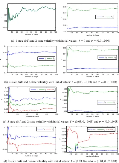
Figure 2.1 shows three plots depicting the evolution of estimates for f, σ and the transition
matrix A under the two-state weak Markov chain setting. For the three-state weak Markov
chain setting, the transition matrix has 33 = 27 elements and their evolutions are shown in
three separate plots in Figure 2.2. Figure 2.3 displays the plots for the dynamics of the mean
and volatility under the 3-state WHMM set-up. In both 2-state and 3-state WHMM modeling
frameworks, the movements of the mean and volatility exhibit similar patterns. It is worth
noting that through this multi-pass recursive algorithm, parameters appear to stabilize after
approximately six passes. Our experiment indicates that this stability is achieved regardless of
the choice of the initial parameter values. We note nonetheless that the speed of convergence
is sensitive to the initial choice of parameter values. We note that on step 140, there is a
change in the trend of the estimated probabilities and kinks in the estimated f and σ. This
coincides with the market crisis that occurred in mid 2008. Thus, the filters are able to adapt
to market conditions that prevailed in that period. We derive the explicit formula of the Fisher
1 10 20 30 40 50 60 70 80 90 100 110 120 130 140 150 160 0
0.2 0.4 0.6 0.8 1
Number of steps
Probabilities
Probabilities with current state=1
a111 a211 a311 a111 a212 a312 a113 a213 a313
1 10 20 30 40 50 60 70 80 90 100 110 120 130 140 150 160 0
0.2 0.4 0.6 0.8 1
Number of steps
Probabilities
Probabilities with current state=2
a121 a221 a321 a122 a222 a322 a123 a223 a323
1 10 20 30 40 50 60 70 80 90 100 110 120 130 140 150 160 0
0.2 0.4 0.6 0.8 1
Number of steps
Probabilities
Probabilities with current state=3
a131 a231 a331 a132 a232 a332 a133 a233 a333
1 10 20 30 40 50 60 70 80 90 100 110 120 130 140 150 160 −0.005
0 0.005 0.01 0.015 0.02 0.025 0.03
Number of steps
f f(1)f(2)
f(3)
1 10 20 30 40 50 60 70 80 90 100 110 120 130 140 150 160 0
0.02 0.04 0.06 0.08 0.1 0.12 0.14 0.16
Number of steps
σ σσ(1)(2)
σ(3)
Parameter Range of standard errors
estimate 1-state 2-state 3-state
ˆ
arst [3.22×10⁻¹⁴, 3.19×10⁻⁹] [1.18×10⁻¹², 1.26×10⁻⁷] [8.21×10⁻¹², 1.25×10⁻⁵]
ˆ
fr [5.18×10⁻¹⁸, 5.74×10⁻¹³] [2.99×10⁻¹⁶, 1.32×10⁻¹⁰] [2.26×10⁻¹⁴, 7.57×10⁻⁹]
ˆ
σr [2.59×10⁻¹⁸, 2.87×10⁻¹³] [1.50×10⁻¹⁶, 6.75×10⁻¹¹] [1.13×10⁻¹⁴, 4.04×10⁻⁹]
Table 2.3: Range of SEs for each parameter under the 1-, 2- and 3-state settings
defined as the negative expectation of the second derivative of the log-density for a parameter
θ. The inverse of the Fisher information is used to calculate the variance associated with the
maximum-likelihood estimates. The sampling distribution of a maximum likelihood estimator
is asymptotically normal and its variance can be calculated from I−1(θ); see Garthwaite, et
al. [10], for example. Following equations (C.1), (C.7) and (C.8) for 1 ≤ r, s, t ≤ N, the
closed-form expressions for the Fisher information of each parameter are given by
I(arst)=
ˆ
Jkrst
a2 rst
, I(fr)=
ˆ
Ork σ−2
r
and I(σr)=−
ˆ
Ork σ2 r
+ 3
ˆ
Tr k(y
2 k)−2 ˆT
r
k(yk)fr+ f 2 r
σ−4 r
.
We provide the range of tabulated SEs over the entire algorithm steps for each parameter in
Table 2.3 under the WHMM withN =1, 2, 3.
Since the model via recursive formulas is self-updating and quickly produces reasonable
pa-rameter estimates, we can use it to forecast asset prices over an h-day ahead horizon. The
semi-martingale representation of a weak Markov chainxin equation (2.5) suggests that
E[ξ(xk+1,xk)|Yk]=Πpk, wherepk =E[ξ(xk,xk−1)|Yk].
This tells us that
E[ξ(xk+h,xk+h−1)
Yk]=Π
h
pk, forh=1,2. . . . (2.30)
Recall thatAis defined byalmv = P(xk+1 =el|xk =em,xk−1 =ev), so that
Equations (2.31) and (2.30) then imply that
E[xk+h|Yk]=Apk+h−1= AΠh−1pk. (2.32)
Using equation (2.32), the best estimate of the logarithmic incrementyk+h given available
in-formation at timekis
E[yk+h|Yk]= hf,AΠh−1pki.
On the other hand, the conditional variance ofyk+his given by
Var[yk+h|Yk]=f >
diag(AΠh−1pk)f+σ >
diag(AΠh−1pk)σ− hf,AΠh −1
pki2,
where diag(AΠh−1pk) is a diagonal matrix whose diagonal entries are the components of the
vectorAΠh−1pk.
Conditional on the information structureYk, the observation processyk+h has a mixed normal
distribution with explicit representation
N
X
i,j=1
hpk+h−1,ei jiφ(y; fi, σi).
Therefore the best estimate of the asset price at time k+h based on available information at
timekis given by
E[Sk+h|Yk]=Sk N
X
i,j=1
hΠh−1pk,ei jiexp fi+
σ2 i
2 !
. (2.33)
Equation (2.33) is used to compute the h-day ahead forecasts of the S&P500 index values.
In a related study, Mamon, et al. [16] compared the predictability performance under the
Diebold-Kilian metric of two- and three-state HMM with the predictability performance
im-plied by their chosen benchmarked models, namely, autoregressive conditional
h−day RMSE AME RAE APE
ahead WHMM HMM WHMM HMM WHMM HMM WHMM HMM
1 14.6652 14.6471 10.4380 10.4249 0.0663 0.0663 0.0092 0.0092
2 20.1931 20.1873 14.8358 14.8329 0.0943 0.0943 0.0130 0.0130
3 23.9568 23.9544 17.8275 17.8331 0.1133 0.1133 0.0157 0.0157
4 27.2519 27.2521 20.3194 20.3276 0.1291 0.1292 0.0179 0.0179
5 30.1839 30.1862 22.4197 22.4284 0.1425 0.1425 0.0197 0.0197
6 32.7025 32.7057 24.4092 24.4189 0.1551 0.1552 0.0215 0.0215
7 34.9630 34.9673 26.0477 26.0606 0.1655 0.1656 0.0229 0.0229
8 36.8720 36.8770 27.4169 27.4313 0.1742 0.1743 0.0241 0.0242
9 38.7440 38.7496 28.6977 28.7143 0.1824 0.1825 0.0253 0.0253
10 40.5210 40.5268 30.0238 30.0416 0.1908 0.1909 0.0265 0.0266 11 42.3122 42.3185 31.4179 31.4378 0.1997 0.1998 0.0278 0.0278 12 43.9374 43.9445 32.6621 32.6803 0.2076 0.2077 0.0289 0.0289 13 45.8010 45.8090 34.1693 34.1893 0.2171 0.2173 0.0303 0.0303 14 47.6995 47.7079 35.7466 35.7676 0.2272 0.2273 0.0316 0.0317 15 49.4687 49.4772 37.0384 37.0573 0.2354 0.2355 0.0328 0.0328 16 51.0220 51.0303 38.2533 38.2738 0.2431 0.2432 0.0339 0.0339 17 52.6908 52.6991 39.5625 39.5788 0.2514 0.2515 0.0350 0.0350 18 54.3287 54.3370 40.7496 40.7646 0.2590 0.2591 0.0361 0.0361 19 55.7159 55.7239 41.8855 41.8977 0.2662 0.2663 0.0371 0.0371 20 57.1569 57.1648 43.0776 43.0913 0.2738 0.2738 0.0381 0.0381 21 58.5421 58.5499 44.0828 44.0959 0.2801 0.2802 0.0390 0.0390 22 59.7281 59.7360 45.0667 45.0793 0.2864 0.2865 0.0399 0.0399 23 61.0026 61.0106 46.0674 46.0786 0.2928 0.2928 0.0409 0.0409 24 62.2606 62.2689 47.1080 47.1190 0.2994 0.2994 0.0418 0.0418 25 63.4862 63.4945 48.0434 48.0530 0.3053 0.3054 0.0426 0.0426
Table 2.4: Error analysis of WHMM and HMM models under the 2-state setting
compared to the benchmarked models, HMM models produce higher measures of short- and
medium-run predictability.
In this empirical implementation, we compare the forecasting performance of WHMM with
that of the regular HMM. The goodness of fit of the h-day ahead forecasts (h = 1, . . . ,25)
to the actual data is evaluated using the root mean square error (RMSE), absolute mean error
(AME), relative absolute error (RAE) and absolute percentage error (APE). These forecasts