finite fields: new upper bounds
Alessandro De Piccoli1, Andrea Visconti2, Ottavio Giulio Rizzo1
1
Department of Mathematics “Federigo Enriques”, Universit`a degli Studi di Milano
[email protected] [email protected]
2
Department of Computer Science “Giovanni Degli Antoni”, Universit`a degli Studi di Milano
[email protected] http://www.di.unimi.it/visconti
Abstract. When implementing a cryptographic algorithm, efficient operations have high relevance both in hardware and software. Since a number of operations can be performed via polynomial multiplication, the arithmetic of polynomials over finite fields plays a key role in real-life implementations. One of the most interesting paper that addressed the problem has been published in 2009. In [5], Bernstein suggests to split polynomials into parts and presents a new recursive multiplication technique which is faster than those commonly used. In order to further reduce the number of bit operations [6] required to multiply n-bit polynomials, researchers adopt different approaches. In [18] a greedy heuristic has been applied to linear straight-line sequences listed in [6]. In 2013, D’angella, Schiavo and Visconti [20] skip some redundant operations of the multiplication algorithms described in [5]. In 2015, Cenk, Negre and Hasan [12] suggest new multiplication algorithms. In this paper, (a) we present a “k-1”-level Recursion algorithm that can be used to reduce the effective number of bit operations required to multiplyn-bit polynomials; and (b) we use algebraic extensions ofF2 combined
with Lagrange interpolation to improve the asymptotic complexity.
Keywords: Polynomial multiplication, Karatsuba, Two-level Seven-way Recursion algorithm,
bi-nary fields, fast software implementations.
1
Introduction
Finite fields have applications in many areas of computer science and engineering, such as digital
signal processing [27,9], coding theory [3,8], cryptography [28,2,10,29,23] and so on. Such
appli-cations usually need efficient implementations both in hardware [32,15,14,1,17,26,24] and software
[5,20,18,12], thus a fast execution of arithmetic operations over finite fields is a crucial issue. In
this paper particular attention is paid to binary fields, i.e., finite fields of characteristic 2, because
they are very attractive for several cryptographic applications, especially for those who play with
elliptic curves [4,7,5].
A binary field F2n is composed of binary polynomials modulo a n-degree irreducible
polyno-mial. The multiplication between two elements ofF2nis one of the most crucial low-level arithmetic
irreducible polynomial. Whereas the modular reduction is a relatively simple operation, the
poly-nomial multiplication turns out to be a costly operation. A real case scenario can help readers to
understand the problem in details. In 2009, Bernstein show that, on a binary Edwards curve [5], a
251-bit single-scalar multiplication requires 44,679,665 bit operations, 43,011,084 of which (about
96%) are for field multiplications. That said, it is not difficult to understand why fast software
implementations for polynomial multiplication over finite fields are desired.
It is well known that the naive polynomial multiplication algorithm — the so-called School-book
algorithm — is not the optimal way to multiply two polynomials. If the polynomials involved in
the product have the same degree, sayn, the multiplication takesn2 multiplications and (n−1)2
additions. Thus, its complexity is 2n2+O(n). Many researchers has tried to improve this algorithm, following two main directions: (1) provide a better asymptotic estimation [32,16,33,22]; (2) reduce
the effective number of bit operations [5,12,14,21,20].
A number of interesting approaches that improves the school-book algorithm have been
pub-lished in literature — see for example Karatsuba [25], Toom [36], Cook [19], Sch¨onhage and Strassen
[35], Bernstein [5], and so on. More precisely, Karatsuba [25] achieves an asymptotic complexity
of 7n1.58+O(n). Toom [36] and Cook [19] reduced the number of steps needed to multiply two
polynomials introducing an algorithm with complexity O(n1+), for arbitrary small >0. In [35]
Sch¨onhage and Strassen showed how to achieved complexityO(nlognlog logn) using a procedure based on the Fast Fourier Transform (FFT). In 2009, Bernstein [5] improves the Karatsuba identity
(Three-way Recursion algorithm), obtaining the following asymptotic complexity 6.5n1.58+O(n). Cenk, Negre and Hasan in [12] suggest to change the field for the polynomials, getting an asymptotic
complexity of 15.125n1.46−2.67nlog
3(n) +O(n).
Notice that asymptotic estimations are not explicit bounds and real-world applications have to
deal with issues of hardware and software implementations — e.g., hardware constraints, software
speedups, and so on. Therefore, in order to get the minimum number of bit operations needed to
multiply twon-bit polynomials — for sake of simplicity we call such a numberM(n) — researchers
analyze, rearrange and modify the algorithms that provide interesting asymptotic estimations.
Their aim is to improve bounds published in literature for specific value (small) of n, and these
improvements that are not visible in the asymptotics. Consequently, a number of papers tries to
reduce the effective number of bit operations [32,16,33,22]. As far as we know, the best explicit
upper bounds for the polynomial multiplication appear in [6,18,20,12].
Karatsuba [25] was the first one who reduces the number of bit operations of the
School-book algorithm. A different approach has been described by Bernstein in 2009 [5]. He refines
the Karatsuba identity and suggests to use a polynomial multiplication technique which employs
(recursively) different multiplication algorithms, picking, at each step, the best one. Moreover, he
presents three new multiplication algorithms — i.e., Three-way Recursion, Five-way Recursion, and
Two-level Seven-way Recursion algorithm — that are useful used to reduce the effective number
of bit operations. The technique presented in [5] not only results in new software speed records [6],
but also avoids well-known software side-channel attacks. Indeed, all computations are expressed
as straight-line sequences of AND/XOR operations, thus they are data-independent. In [18] are
published improvements for specific value ofnobtained by applying Boyar-Peralta heuristic [11] on
the linear part of straight-line sequences reported in [6]. In 2013, D’angella, Schiavo and Visconti
[20] skip some redundant operations of the multiplication algorithms described in [5], reducing
the number of bit operations for many values of n. The authors focus in particular on Five-way
present new multiplication algorithms which improve many of the explicit upper bounds previously
described.
1.1 Our contributions
In this paper we investigate the possibility to (a) further reduce the effective number of bit
opera-tions required to multiplyn-bit polynomials, and (b) improve the asymptotic complexity.
Firstly, we refine the Two-level Seven-way Recursion algorithm [5]. As shown in [5], it seems
that Lagrange Interpolation is a useful tool to arrange the order of operations. Although in many
cases this is true, in others it is not. Rearranging the operations in a different way, we present a
“k-1”-level Seven-way Recursion algorithm, or“k-1”-level Recursion for short. We show thatThree-,
Four-, and Five-level Recursion can be used to improve the explicit upper bounds published in
literature.
Secondly, we use algebraic extensions ofF2 combined with Lagrange interpolation to improve
the asymptotic complexity. We will show an interesting connection between this technique and the
computation of the values of a polynomial in all of the field elements.
1.2 Organization of the paper
The remainder of the paper is organized as follows. In Section 2, we state definitions and some
preliminary concepts that are useful to understand the following sections. In Section 3, starting
with the classical school-book algorithm, we introduce some of the approaches currently adopted
to multiply polynomials in an efficient way. The Section 4 is the heart of this paper. We present
our contribution, showing the new speed records achieved and explaining the techniques adopted.
Finally, conclusions are drawn in Section 5.
2
Preliminaries
We restrict our analysis to polynomials over finite fields of characteristic 2, so we will not ever use
the minus sign. IfF(t) andG(t) are two of these polynomials, we will call their productH(t).
To denote the cost of the multiplication inFg between two polynomials of degreen−1 we will
useMg(n).
2.1 Projective Lagrange Interpolation
As pointed out in [12], Lagrange Interpolation leads us to efficient multiplication algorithms. How
does this technique work? Consider a fieldKand a polynomialH ∈K[x],
H(x) =h0+h1x+h2x2+...+hnxn
Algebra tells us that we need to fix the value of the polynomial inn+ 1 points in order to uniquely
determine it. So, given a set of n+ 1 distinct points {k0, . . . , kn} ⊆ K, we define the Lagrange polynomials as follows:
li(x) = Y
j6=i
x−kj
ki−kj
Notice that we haveli(ki) = 1 andli(kj) = 0,∀j6=i. This feature allows us to exactly reconstruct
any polynomial H ∈K[x] as
H(x) =
n X
i=0
H(ki)·li(x)
For our purposes, the above technique is not optimal. Given the same problem with onlynpoints
{k0, ..., kn−1}, define the degreen−1 polynomial
H =
n−1 X
i=0
H(ki)·li(x)
We still have H(ki) =H(ki), fori= 0, ..., n−1. Let
l∞(x) = n Y
j=0
(x−ki)
and H(∞) =hn. SinceH(∞)·l∞ vanishes at every ki and has degreen, we can reconstruct H
with the so-called Projective Lagrange Interpolation formula,
H(x) =
n−1 X
i=0
H(ki)·li(x) +H(∞)·l∞.
2.2 Which field?
Lagrange Interpolation requiresn+1 points, but we just have two points inF2! Projective Lagrange
Interpolation will do with n points since it makes use of the point at infinity: where can we find
even more points? A possible answer is to consider finite algebraic extensions of F2, generated
by a monic irreducible polynomial γ over F2 of degree d. Indeed, an extension F is a quotient
F2[X]/hγ(X)i, so the elements ofFare all d-bit polynomials, i.e., the set of polynomials overF2
of degree at most d−1, andF has 2d elements. If δ is another irreducible polynomial of degree
d, there is a, non canonical, isomorphism F2[X]/hγ(X)i 'F2[X]/hδ(X)i, so we will call such an
extensionF2d.
F×2d is a cyclic group: letαbe a fixed generator, we can seeF2d as a vector space overF2 with
basis{1, α, α2, . . . , αd−1}. At last, note that
F2d is the splitting field ofX2 d
+X: its roots are all
the elements of the field.
3
Current approaches
3.1 School-book algorithm
Given twon-bit polynomials
F=f0+f1t+...+fntn and G=g0+g1t+...+gntn.
The steps of the algorithm are:
– Recursively multiplyf0+f1t+...+fn−1tn−1byg0+g1t+...+gn−1tn−1;
– Compute (fng0+f0gn)tn+ (fng1+f1gn)tn+1+...+fngnt2n. This takes 2n+ 1 multiplications
– Add the former to the latter. This takesn−1 additions for the coefficients oftn, ..., t2n−2; the
other coefficients do not overlap.
We get the recursion formula M(n+ 1) ≤ M(n) + 4n and the asymptotic estimation M(n) ≤
2n2−2n+ 1. This algorithm is efficient only in low degrees. Indeed, as reported in [6], the cost of
the school-book algorithm is too high from degree 14 on.
3.2 Karatsuba
Given two 2n-bit polynomialsF andG, write them asF =F0+F1tn,G=G0+G1tn for some
other n-bit polynomials F0, F1, G0, G1. The Karatsuba algorithm [25] can be described by the
product.
(F0+tnF1)(G0+tnG1)
= (1 +tn)F0G0+tn(F0+F1)(G0+G1) + (tn+t2n)F1G1
The operations involved are:
– M2(n): multiplicationF0G0
– n−1: sum S1= (1 +tn)F0G0 – 2n: sumsF0+F1,G0+G1
– M2(n): multiplication (F0+F1)(G0+G1)
– M2(n): multiplicationF1G1
– n−1: sum S2= (tn+t2n)F1G1
– 2n−1: sumS3=S1+tn(F0+F1)(G0+G1) – 2n−1: sumS3+S2
Summing all costs, we get
M2(2n)≤3M2(n) + 8n−4 (1)
3.3 Bernstein
Bernstein improves the Karatsuba algorithm defining the so-called Refined Karatsuba algorithm
[5]. As described in Section 3.2, we consider two 2n-bit polynomialsF,Gand takeF0,G0asn-bit
polynomials andF1, G1 ask-bit polynomials. The Refined Karatsuba algorithm can be described
as follows.
(F0+tnF1)(G0+tnG1)
= (1 +tn)F
0G0+tn(F0+F1)(G0+G1) + (tn+t2n)F1G1
= (1 +tn)F0G0+tn(F0+F1)(G0+G1) + (1 +tn)tnF1G1
= (1 +tn)(F
0G0+tnF1G1) +tn(F0+F1)(G0+G1)
The cost estimation of the algorithm is
M2(n+k)≤2M2(n) +M2(k) + 4k+ 3n−3 n/2≤k≤n (2)
This improves that of Karatsuba described in Section 3.2.
Moreover in [5] we can find another improvement but for higher degrees. In fact, Bernstein
polynomial of 4n bits. Applying the Refined Karatsuba identity three times and factoring out
1 +tn, we get
(F0+tnF1+t2nF2+t3nF3)(G0+tnG1+t2nG2+t3nG3)
= (1 +t2n)
(1 +tn)(F
0G0+tnF1G1+t2nF2G2+t3nF3G3)
+tn(F
0+F1)(G0+G1) +t3n(F2+F3)(G2+G3)
+t2n(F
0+F2+tn(F1+F3))(G0+G2+tn(G1+G3))
The cost evaluation for polynomials with 3n+kcoefficients, assumingn/2≤k≤n, is
– 3M(n): multiplicationsF0G0,F1G1, F2G2.
– M(k): multiplicationF3G3.
– 3(n−1): sumsS1=F0G0+tnF1G1+t2nF2G2+t3nF3G3. – 2n+ 2k−1: sum (1 +tn)S
1.
– 2n+M(n): multiplicationS2= (F0+F1)(G0+G1).
– 2k+M(n): multiplicationS3= (F2+F3)(G2+G3).
– 4n−2: sums S4= (1 +tn)S1+tnS2+t3nS3.
– 2n+ 2k+M(2n): multiplicationS5= (F0+F2+tn(F1+F3))(G0+G2+tn(G1+G3)).
– 6n+ 2k−2: sum (1 +t2n)S4+t2nS5.
Hence, summing all the costs, we obtain
M(3n+k)≤M(2n) + 5M(n) +M(k) + 19n+ 8k−8 n/2≤k≤n (3)
3.4 Cenk, Negre, Hasan
In [12] and [13], the authors suggest to use a field bigger than F2 for Projective Lagrange
In-terpolation. They consider two 3n-bit polynomials F and G, written as F =F0+F1tn+F2t2n,
G=G0+G1tn+G2t2n withF0,F1,F2,G0,G1,G2 n-bit polynomials. Then, they make
compu-tations using the elements ofF4. Ifαis a generator ofF×4, and assumingnodd, the new algorithm
can be written as follows.
H(t) = (F0+tnF1+t2nF2)(G0+tnG1+t2nG2)
H(0) =F0G0
H(1) = (F0+F1+F2)(G0+G1+G2)
H(α) = (F0+F2+α(F1+F2))(G0+G2+α(G1+G2))
H(α+ 1) = (F0+F1+α(F1+F2))(G0+G1+α(G1+G2))
H(∞) =F2G2
(F0+tnF1+t2nF2)(G0+tnG1+t2nG2)
= (H(0) +tnH(∞))(1 +t3n) + (H(1) + (1 +α)(H(α) +H(α+ 1)))
+(H(1) + (1 +α)(H(α) +H(α+ 1)))(tn+t2n+t3n)
+α(H(α) +H(α+ 1))t3n+H(α)t2n+H(α+ 1)tn
(4)
Notice that if nis even, we just exchange the formulae for H(α) andH(α+ 1). As described in
M2(3n)≤2M4(n) + 3M2(n) + 29n−12
An improvement of this algorithm is described in [12]: using two polynomialsC0andC1to rearrange
equationsH(α) andH(α+ 1)
H(α) = (F0+F2+α(F1+F2))(G0+G2+α(G1+G2)) =C0+αC1
H(α+ 1) = (F0+F1+α(F1+F2))(G0+G1+α(G1+G2)) = (C0+C1) +αC1
it is possible to redefine (4) as
(F0+tnF1+t2nF2)(G0+tnG1+t2nG2)
=H(∞)t4n+H(0)
+(H(0) +H(1) +C1)t3n+ (C0+H(1) +C1)t2n+ (H(∞) +H(1) +C0)tn.
The relative cost for this algorithm is
M2(3n)≤3M2(n) +M4(n) + 20n−5
M4(3n)≤5M4(n) + 56n−19
(5)
However, 5 does not perform well for low degrees as shown in [12] (see table 2). More encouraging
is the asymptotic estimation, but it requires the following two lemmas.
Lemma 1. Let a,b andi be positive integers and assume thata6=b. Let n=bi anda6= 1. The solution to the inductive relation
r1=e
rn=arn/b+cn+d
is
rn=
e+ bc
a−b + d a−1
nlogba− bc
a−bn− d a−1.
Proof. The proof is trivial. Substituting in the inductive relation the expression for rn and rn/b,
we find an identity.
Lemma 2. Let a,b andi be positive integers. Let n=bi and a=b and a6= 1. The solution to the inductive relation
r1=e
rn =arn/b+cn+f nδ+d
is
rn =
e+ f b
δ
a−bδ +
d a−1
n−nδ
f bδ a−bδ
+cnlogbn−
d a−1.
Proof. Similar to the previous one
Going back to (5), we can apply the first lemma to the second inequality, getting
M4(n)≤30.25n1.46−28n+ 4.75
M2(3n)≤3M2(n) + 30.25n1.46−8n−0.25
Finally, using the second lemma we get the asymptotic estimation
M2(n)≤15.125n1.46−14.25n−2.67nlog3n+ 0.125.
4
Our contribution
In this Section, we define a more efficient algorithm rearranging the order of operations and improve
the general complexity through asymptotic estimations. In the sequel, we will denote these two
approaches with(I)and(II)respectively.
4.1 Improvements of Two-level Seven-way (I)
We can now give an improvement of the preceding algorithm for higher degrees. In fact, we consider
polynomials of 8n bits and apply the same technique of the Two-level Seven-way Recursion. We
can collect t4n, apply the Refined Karatsuba and apply Two-level Seven-way Recursion for inner
multiplication. We will call the following algorithm Three-level Recursion.
P7 i=0t
inF
i P7i=0tinGi
=P3i=0tinFi+t4n P3
i=0t inF
i+4 P3
i=0t inG
i+t4n P3
i=0t inG
i+4
= (1 +t4n)P3 i=0t
inF i
P3 i=0t
inG i
+t4nP3 i=0t
inF i+4
P3 i=0t
inG i+4
+
t4nP3 i=0t
inF
i+P3i=0tinFi+4 P3i=0tinGi+P3i=0tinGi+4
= (1 +t4n)P3i=0tinFi P3
i=0t inG
i
+t4nP3i=0tinFi+4 P3
i=0t inG
i+4
+
t4nP3 i=0t
in(F
i+Fi+4) P3
i=0t in(G
i+Gi+4)
= (1 +t4n)((1 +t2n)((1 +tn)P7 i=0t
inF iGi
+
P3 j=0t
(2j+1)n(F
2j+F2j+1)(G2j+G2j+1))+
+t2n(F
0+F2+ (F1+F3)tn)(G0+G2+ (G1+G3)tn)+
+t6n(F4+F6+ (F5+F7)tn)(G4+G6+ (G5+G7)tn))+
t4nP3 i=0t
in(F
i+Fi+4) P3
i=0t in(G
i+Gi+4)
The cost evaluation for polynomials with 7n+kcoefficients, assumingn/2≤k≤n, is
– 7M(n): multiplicationFiGi, fori= 0, . . . ,6
– M(k): multiplicationF7 byG7
– 7(n−1): sumS1=P7i=0tinFiGi – 6n+ 2k−1: sum S2= (1 +tn)S1
– 2k+M(n): multiplication (F6+F7)(G6+G7)
– 4(2n−1): sumS3=S2+ P3
j=0t
(2j+1)n(F
2j+F2j+1)(G2j+G2j+1) – 6n+ 2k−1: sumS4= (1 +t2n)S3
– 4n+M(2n): multiplicationS5= (F0+F2+ (F1+F3)tn)(G0+G2+ (G1+G3)tn)
– 2n+ 2k+M(2n): multiplicationS6= (F4+F6+ (F5+F7)tn)(G4+G6+ (G5+G7)tn)
– 2(4n−1): sumS7=S4+t2nS5+t6nS6 – 6n+ 2k−1: sumS8= (1 +t4n)S7 – 6n+ 2k+M(4n): multiplicationS9=
P3 i=0t
in(F
i+Fi+4) P3
i=0t in(G
i+Gi+4)
– 8n−1: sumS8+t4nS9
Hence, summing all the costs, we get
M(7n+k)≤M(4n) + 2M(2n) + 11M(n) +M(k) + 67n+ 12k−17 n/2≤k≤n
One could continue in the same fashion of theThree-level, consider polynomials of 2knbits, collect
t2k−1n, apply the Refined Karatsuba and the “k-1”-level Recursion. We are going to see that this
is not a totally right way.
We want to see which kind of improvements are given from algorithms of the Section 3.3. They
are of two types: asymptotic and concrete (only on low degree). Lemma 1 will help us to state
asymptotic estimations.
If we go back to the recursion (2), we see that, whenkis equal ton, it could be rewritten as
M(2n)≤3M(n) + 7n−3 (6)
so, also as
M(n)≤3M(n/2) +7 2n−3. We can now apply Lemma 1, finding
M(n)≤6.5nlog23−7n+ 1.5 What about (3)? If we statek=n, we get
M(4n)≤M(2n) + 6M(n) + 27n−8
so, we cannot apply Lemma 1, but if we substituteM(2n) with the recursion formula 6, we find
M(4n)≤9M(n) + 34n−11
finally, we obtain
M(n)≤6.43nlog23−6.8n+ 1.38
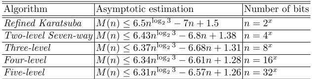
To enable an easy comparison of different algorithms, in Table 1 we present the asymptotic
estimations. Notice that the first and the third coefficients of each estimation are decreasing,
instead the second one is growing.
By exploiting the recursion formulae, we can also improve the cost of the multiplication between
Algorithm Asymptotic estimation Number of bits
Refined Karatsuba M(n)≤6.5nlog23−7n+ 1.5 n= 2x Two-level Seven-wayM(n)≤6.43nlog23−6.8n+ 1.38 n= 4x
Three-level M(n)≤6.37nlog23−6.68n+ 1.31n= 8x Four-level M(n)≤6.34nlog23−6.61n+ 1.28n= 16x Five-level M(n)≤6.31nlog23−6.57n+ 1.26n= 32x
Table 1.Asymptotic estimations: comparison of different algorithms
n Best known De Piccoli Algorithm used Gain
(2017)
24 702 [12] 697 3-lev 5
32 1156 [12] 1148 3-lev 8
39 1680 [12] 1677 3-lev 3
40 1718 [12] 1705 3-lev 13
47 2229 [12] 2214 3-lev + 4-lev 5+10
48 2260 [12] 2238 3-lev + 4-lev 8+14
56 3060 [5] 3042 3-lev 18
63 3632 [12] 3612 3-lev + 4-lev 2+18
64 3674 [12] 3636 3-lev + 4-lev + 5-lev 13+21+4
71 4476 [12] 4473 3-lev 3
72 4535 [12] 4511 3-lev 24
79 5359 [12] 5328 3-lev + 4-lev 19+12
80 5400 [12] 5360 3-lev + 4-lev 20+20
95 7073 [12] 6965 3-lev + 4-lev + 5-lev 45+24+39
96 7112 [12] 6993 3-lev + 4-lev + 5-lev 51+25+43
120 10438 [5] 10352 3-lev 86
126 11346 [5] 11220 3-lev + 4-lev + 5-lev 38+29+59
127 11447 [5] 11248 3-lev + 4-lev + 5-lev 104+24+71
128 11466 [12] 11280 3-lev + 4-lev + 5-lev 74+38+74
Table 2.Improvements ofM(1)−M(128): we apply Three-, Four-, and Five-level Recursion algorithm
4.2 Product in finite fields: general case (II)
There are several approaches that can be adopted to multiply two polynomials, sayF andG, in an
efficient way. In this section we provide a new one. In doing so, we make some useful assumptions.
We takeda non negative integer and the factors F andGof the form
F(t) =
2d−1 X
i=0
Fi(t)tin withFi∈F2[t], degFi ≤n−1
In order to simplify notation, given a factorF(t) of the above form, we define
e
F(x) =
2d−1
X
i=0
Fi(t)xi
We are now ready to suggest a new efficient algorithm.
Let’s start with an observation. There is an interesting connection betweenx2d+xand Lagrange
polynomials. Indeed, we can prove the following three equalities:
1. l0(x) =
x2d
+x x =x
2d−1
2. lαi(x) =
x2d
+x
x+αi i= 0,1, . . . ,2 d−2
3. l∞=x2
d
+x=x(x2d−1+ 1) =x·l 0(x)
We now rewrite the interpolation law as follows:
e
H(x) =He(0)·l0(x) + 2d−2
X
i=0 e
H(αi)·lαi(x) +He(∞)·l∞(x)
e
H(x) =He(0)·l0(x) + 2d−2
X
i=0 e
H(αi)·lαi(x) +xHe(∞)·l0(x)
e
H(x) =He(0)·(1 +x2
d−1
) +
2d−2 X
i=0 e
H(αi)x
2d+x
x+αi +xHe(∞)·(1 +x 2d−1
)
e
H(x) = (1 +x2d−1)(He(0) +xHe(∞)) + 2d−2
X
i=0 e
H(αi)x
2d+x
x+αi (7)
Notice that fractions x2
d
+x
x+αi of Equation 7 are Lagrange polynomials ofF
×
2d. Using the naive division
algorithm, we obtain
lαi(x) =
x2d+x x+αi =
2d−1
X
j=1
(αi)(j−1)x2d−j (8)
and replacing Equation 8 in 7, we get
e
H(x) = (1 +x2d−1)(He(0) +xHe(∞)) + 2d−2
X
i=0 e
H(αi)
2d−1
X
j=1
αi(j−1)x2d−j
e
H(x) = (1 +x2d−1)(He(0) +xHe(∞))
| {z }
SA
+
2d−1
X
j=1
2d−2
X
i=0
αi(j−1)He(α i
)
x 2d−j
| {z }
SB
(9)
We will now discuss the costs of this algorithm.
Consider SA: it will always be the same in every fieldF2d. The cost of the operations inSAis:
– M2(n): multiplicationHe(0) =F0G0
– M2(n): multiplicationHe(∞) =F2d−1G2d−1
– n−1: sum He(0) +xHe(∞)
– 0: sum (1 +x2d−1)(He(0) +xHe(∞))
The last estimate holds only ford6= 1, otherwise polynomialsHe(0)+xHe(∞) andx(He(0)+xHe(∞))
overlap on some bits and it becomes 2n−1.
Consider now the sumSA+SB. The degree ofSAis (2d+ 2)n−2, but its structure lacks many
powers. Indeed,SA is a polynomial that has two parts, the first with powers whose degrees are
running from 0 to 3n−2, the second from (2d−1)nto (2d+ 2)n−2. This is very useful because
SB has powers with degrees from nto (2d+ 1)n−2, so,SA and SB overlaps only in two parts.
– 4n−2: sum H(t) =SA+SB
Finally, consider the sums inSB. Supposing that the internal summation has been computed,
the external one is conducted over 2d−1 polynomials. These polynomials have powers fromcn to
cn+ 2n−2, withc= 1, . . . ,2d−1 and each one overlaps the following onn−1 bit. Therefore, the
cost of the external sum in SB is
– (2d−2)(n−1): sumS
1x+S2x2+· · ·+S2d−1x2 d−1
We are left to compute the internal sums inSB. We will show that we do not need to compute all
e
H(αi).
Firstly, we start with showing that ifi= 2qi0for someq, then there will be a connection between
the coefficients of He(αi) andHe(αi
0 ).
Theorem 1. If we take integers i and i0 such that i0 = 2qi for some q, then we can express the
coefficients of He(αi
0
)as a linear combination of the coefficients of He(αi).
Proof. We have
e
H(αi) =Fe(αi)·Ge(αi) = 2d−1
X
j=0
Fjαij 2d−1
X
k=0
Gkαik= 2d X
l=0
X
j+k=l 0≤j,k≤2d−1
FjGk
(αi)l.
We define
Hl= X
j+k=l 0≤j,k≤2d−1
FjGk
thus
e
H(αi) =
2d
X
l=0
Hlαil (10)
Remember that the fieldF2dcan be viewed as vector space over F2. So, we can write every power
ofαas a linear combination of the elements of the basis{1, α, α2, . . . , αd−1}
αil=
d−1 X
b=0
cb,ilαb (11)
and substitute 11 in 10, getting
e
H(αi) =
2d X
l=0
Hl d−1 X
b=0
cb,ilαb= d−1 X
b=0
2d X
l=0
Hlcb,il
α b
Take now He(αiw) withw >1, from (11) we have
αilw= (αil)w=
d−1 X
b=0
cb,ilαb !w
In order to write coefficients ofHe(αiw) as linear combinations of the coefficients ofHe(αi), we need
the following equality:
d−1 X
b=0
cb,ilαb !w
=
d−1 X
b=0
cb,ilαbw (12)
Suppose it holds, then
e
H(αiw) =
2d X
l=0
Hl d−1 X
b=0
cb,ilαb !w
=
2d X
l=0
Hl d−1 X
b=0
cb,ilαbw= d−1 X
b=0
2d X
l=0
Hlcb,il
α bw.
Finally, using (11), we obtain
e
H(αiw) =
d−1 X
b=0
2d X
l=0
Hlcb,il
α bw=
d−1 X
b=0
2d X
l=0
Hlcb,il
d−1 X
t=0
ct,bwαt=
=
d−1 X
t=0
d−1 X
b=0
ct,bw
2d
X
l=0
Hlcb,il
αt
Let’s go back to (12): since we are in characteristic two, the equality holds whenw= 2q, for some
q.
Secondly, we have to remember thatα2d=α. So, for every e
H(αi), withi6≡0 mod 2d−1, there
are at mostddifferent evaluations ofHe that can be computed withHe(αi). They are the following
set:
Pi={He(αi),He(α2i),He(α2
2i
), . . . ,He(α2
d−1i )}
We can count the number ofPi for every algebraic extension ofF2, because it depends only on the
degreed.
Theorem 2. The number of differentPi is
P =−1 + 1
d
d−1 X
k=0
gcd(2k−1,2d−1)
In particular, if2d−1 is prime, P = (2d−2)/d.
We define an action of the (additive) groupZonZ/(2d−1)Zas k·i= 2ki. Sincedacts trivially, this action induces an action of Z/dZ on Z/(2d−1)
Z: if O(i) is the orbit of i ∈ Z/(2d−1)Z, thenPi={He(αj) :j ∈O(i)}. We have a trivial orbitO(0) ={0}which would correspond to the
set P0 ={He(1)} which we will not count. In order to prove the Theorem 2, we need a couple of
additional lemmata.
Lemma 3 (Burnside’s Lemma).If the finite groupGacts on the finite setX, then the number
of orbits is
1 #G
X
g∈G
# Fix(g)
Proof. See [34], chapter 3.
Lemma 4. Fix an integer N and letx∈Z/NZ. Then
#{y∈Z/NZ:xy= 0}= gcd(x, N)
Proof. LetZ={y∈Z/NZ:xy= 0}: it is not empty since it includes 0 and it is straightforward to verify that Z is an ideal in Z/NZ, thus Z = hdi where d is a divisor of N and Z has N/d elements. Let D = gcd(x, N), ν = N/D and define ˜x as the smallest positive integer such that
˜
x≡xmodN. Since
νx= N
Dx≡N
˜
x
D ≡0 modN
we have that ν ∈ Z. Viceversa, if y ∈ Z and ˜y is the smallest positive integer such that ˜y ≡
ymodN, we have that ˜yx˜=kN for some integerk≥0. Thus
˜
yx˜ D =k
N
D =kν; i.e., y˜
˜
x
D ≡0 modν
Since ˜x/D and ν = N/D are relatively prime, this implies ˜y ≡ 0 modν, i.e., ν divides ˜y, thus
y∈ hνi. This shows thatZ=hνi, hence that #Z=N/ν = gcd(x, N).
Proof (Theorem 2). Fix k∈Z/dZ: we want to compute Fix(k) = {x∈Z/(2d−1)
Z:k·x=x}. If x∈Fix(k) then 2kx=x, that is (2k−1)x= 0; and, viceversa, if (2k−1)x= 0 then k·x=x. Hence, Fix(k) ={x∈Z/(2d−1)Z: (2k−1)x= 0}has, by the previous lemma, gcd(2k−1,2d−1) elements.
The thesis now follows from Burnside’s Lemma.
Let’s sum up the costs of Equation 9.
– M2(n): multiplicationHe(0) =F0G0
– M2(n): multiplicationHe(∞) =F2d−1G2d−1
– n−1: sumHe(0) +xHe(∞) – 0: sum (1 +x2d−1)(
e
H(0) +xHe(∞)) – 4n−2: sum H(t) =SA+SB
– (2d−2)(n−1): sumsS1x+S2x2+· · ·+S2d−1x2 d−1
– ∆1: evaluationFe(αi),Ge(αi)
– M2(n): multiplicationHe(1)
– P M2d(n): multiplicationsHe(αi)
– ∆2: sumsSi,i= 1, . . . ,2d−1
Some of the previous costs are left blank, in particular ∆1 and ∆2, since the evaluation of F,G
and the sumsSi depends on the polynomial used to generate the fieldF2d. Roughly speaking, we
can say that∆1=Anand∆2=B(2n−1), obtaining the following estimation:
M((2d−1+ 1)n)≤3M2(n) +P M2d(n) + (2d+ 3 +A+ 2B)
| {z }
Q1
n+ (−1−2d−B)
| {z }
Q2
M((2d−1+ 1)n)≤3M2(n) +P M2d(n) +Q1n+Q2 (13)
Theorem 3. Let a and b be positive real numbers witha≥1 andb≥2. LetT(n)be defined by
T(n) =
aTln b
m
+f(n) n >1
d n= 1
Then
1. iff(n) =Θ(nc)wherelogba < c, thenT(n) =Θ(nc) =Θ(f(n)), 2. iff(n) =Θ(nc)wherelog
ba=c, thenT(n) =Θ(nlogbalogbn), 3. iff(n) =Θ(nc)wherelog
ba > c, thenT(n) =Θ(nlogba).
The same results apply with ceilings replaced by floors.
Proof. See [30], Section 5.2.
We cannot apply Theorem 3 to 13 since both M2 and M2d appear: we will have to move
everything down toF2-operations.
4.3 Bit operations and asymptotic estimation (II)
As seen in Section 4.2, we need to evaluate anF2d-polynomialFe of degree 2d−1. Recall that the
fieldF2d can be seen as anF2-vector space of dimensiond. Thus, for all i, we can evaluateFe(αi)
as follows:
e
F(αi) =
d−1 X
j=0
Fjαj Fj∈F2[t]
To computeHe(αi) we need to multiply the two evaluations of Fe andGe.
e
H(αi) =Fe(αi)Ge(αi) = d−1 X
j=0
Fjαj d−1 X
k=0
Gkαk = 2d−2
X
l=0
X
j+k=l 0≤j,k≤d−1
FjGk
| {z }
Hl
αl
We want now to computeHl. We take care only of multiplications. If we look atHl, we note that
it is formed by the sum of the products betweenFj andGk such that j+k=l. We separate the
two cases: j = k and j 6= k. If j =k, we need the multiplication FjGj. If j 6=k, we need two
multiplications, which are FjGk and FkGj. For the latter, we exchange one multiplication with
four sums, since charF2d= 2 and we have already computedFjGj.
FjGk+FkGj= (Fj+Fk)(Gj+Gk) +FjGj+FkGk
The required multiplications are
d+
d
2
=d+d(d−1)
2 =
d2+d
2 .
Now, we can write the estimation for bit calculations overF2d, assuming a generic estimate for the
number of bit additions¿
M2d(n)≤
d2+d
Substituting 14 in the estimation 13, we obtain a formula which we can apply Theorem 3 to:
M2((2d−1+ 1)n)≤3M2(n) +P
d2+d
2 M2(n) +Cn+D
+Q1n+Q2
M2((2d−1+ 1)n)≤
3 + P(d
2+d)
2
M2(n) + (Q1+CP)n+ (Q2+DP)
Applying the third case of Theorem 3, we get:
M2(n) =Θ nE, where E=
log3 +P(d22+d)
log(2d+ 1)
If we compute the exponentE for 1≤d≤20, it is not difficult to see thatE decreases from 1.58 to 1.17.
4.4 Case d=2 (II)
Using Equation 9, we are able to find a better asymptotic estimation than that presented in [12]
(see CNH 3-way split algorithm (24)). Indeed,
– M2(n): multiplicationHe(0) =F0G0
– M2(k): multiplicationHe(∞) =F2G2 – 2k: sumsS1=F0+F2,S2=G0+G2
– 2k: sumsS3=F1+F2,S4=G1+G2
– 2n: sumsS5=S1+F1,S6=S2+G1
– 0: multiplicationsP1=αS3,P2=αS3
– 0: sumsS7=S1+P1,S8=S2+P2
– M2(n): multiplicationHe(1) =S5S6
– M4(n): multiplicationHe(α) =S7S8(=C0+C1α)
– 2n−1: sum S9=He(1) +C1 – 2n−1: sum S10=S9+C0 – 2n−1: sum S11=S10+C1
– 2(n−1): sumsS12=S9x3+S10x2+S11x – n−1: sumS13=He(0) +xHe(∞)
– 0: sumS14= (1 +x3)S13
– 4n−2: sum H=S14+S12
Summing all the costs, we obtain
M(2n+k)≤2M2(n) +M2(k) +M4(n) + 15n+ 4k−8 n/2≤k≤n
M(3n)≤3M2(n) +M4(n) + 19n−8 k=n
(15)
But this is not enough. In order to get the asymptotic estimation, we have to compute the costs for
the same algorithm that uses polynomials over F4. In this case, we cannot deduce the expression
forHe(α+ 1) fromHe(α). In addition, from equation
α(a0+a1α) =a1+ (a0+a1)α
(a0+a1α) + (b0+b1α) = (a0+b0) + (a1+b1)α
we have that the cost of the sum between two polynomials is doubled. Thus,
– M4(n): multiplicationHe(0) =F0G0
– M4(n): multiplicationHe(∞) =F2G2 – 4n: sumsS1=F0+F1,S2=G0+G1
– 4n: sumsS3=F1+F2,S4=G1+G2
– 2n: multiplicationsP1=αS3,P2=αS4
– 4n: sumsS5=S1+P1,S6=S2+P2
– 4n: sumsS7=S5+S3,S8=S6+S4
– 4n: sumsS9=S1+F2,S10=S2+G2
– M4(n): multiplicationHe(1) =S9S10
– M4(n): multiplicationHe(α) =S7S8
– M4(n): multiplicationHe(α+ 1) =S5S6
– 6n−3: sumS13=He(1) +He(α) +He(α+ 1)
– 6n−3: sumS14=He(1) +He(α+ 1) +α(He(α) +He(α+ 1)) – 4n−2: sumS15=He(1) +He(α) +α(He(α) +He(α+ 1)) – 2(n−1): sumsS16=S13x3+S14x2+S15x
– n−1: sum S17=He(0) +xHe(∞) – 0: sumS18= (1 +x3)S17
– 4n−2: sumH =S18+S16
The sum of the costs inF4 is
M4(3n)≤5M4(n) + 45n−13 (16)
Applying Lemma 1 to 16, we get
M4(n)≤26.25n1.46−22.5n+ 3.25
Then, we substitute the preceding inequality to the second of 15 obtaining
M2(3n)≤3M2(n) + 26.25n1.46−3.5n−4.75
Finally, to get the asymptotic estimation, we apply Lemma 2:
M2(n)≤13.125n1.46−1.17nlog3n−14.5n+ 2.375.
5
Conclusions
In this paper, we presented a new algorithm to multiply two n-bit polynomials. We showed how
this new approach can be used to (a) reduce the effective number of bit operations and (b) improve
the asymptotic estimations.
The idea described in this paper can be easily implemented to speed up cryptographic software
implementations. Notice that further improvements might be obtained avoiding some redundant
a greedy heuristic [31,11,37] to a straight-line sequence such as the one provided in Appendix A.
Unfortunately, this approach is computational expensive and often it does not provide a useful
result in an acceptable amount of time.
References
1. Abdulrahman, E.A.H., Reyhani-Masoleh, A.: High-speed hybrid-double multiplication architectures using new serial-out bit-level mastrovito multipliers. IEEE Transactions on Computers 65(6), 1734– 1747 (2016)
2. Agnew, G.B., Beth, T., Mullin, R.C., Vanstone, S.A.: Arithmetic operations in GF(2m). Journal of Cryptology 6(1), 3–13 (1993)
3. Berlekamp, E.R.: Algebraic coding theory, vol. 111. McGraw-Hill New York (1968)
4. Bernstein, D.J.: Curve25519: New diffie-hellman speed records. In: Yung, M., Dodis, Y., Kiayias, A., Malkin, T. (eds.) Public Key Cryptography - PKC 2006: 9th International Conference on Theory and Practice in Public-Key Cryptography, New York, NY, USA, April 24-26, 2006. Proceedings, pp. 207–228. Springer Berlin Heidelberg, Berlin, Heidelberg (2006)
5. Bernstein, D.J.: Batch binary edwards. In: Halevi, S. (ed.) Advances in Cryptology - CRYPTO 2009: 29th Annual International Cryptology Conference, Santa Barbara, CA, USA, August 16-20, 2009. Proceedings, pp. 317–336. Springer Berlin Heidelberg, Berlin, Heidelberg (2009)
6. Bernstein, D.J.: High-speed cryptography in characteristic 2: Minimum number of bit operations for multiplication (2009),http://binary.cr.yp.to/m.html
7. Bernstein, D.J., Duif, N., Lange, T., Schwabe, P., Yang, B.Y.: High-speed high-security signatures. Journal of Cryptographic Engineering 2(2), 77–89 (2012)
8. Blahut, R.E.: Theory and practice of error control codes, vol. 126. Addison-Wesley Reading Mas-sachusetts (1983)
9. Blahut, R.E.: Fast algorithms for digital signal processing. Addison-Wesley Longman Publishing Co., Inc. (1985)
10. Blake, I., Seroussi, G., Smart, N.: Elliptic curves in cryptography, vol. 265. Cambridge university press (1999)
11. Boyar, J., Peralta, R.: A new combinational logic minimization technique with applications to cryp-tology. In: Festa, P. (ed.) Experimental Algorithms: 9th International Symposium, SEA 2010, Ischia Island, Naples, Italy, May 20-22, 2010. Proceedings, pp. 178–189. Springer Berlin Heidelberg, Berlin, Heidelberg (2010)
12. Cenk, M., Hasan, M.A.: Some new results on binary polynomial multiplication. Journal of Crypto-graphic Engineering 5(4), 289–303 (2015)
13. Cenk, M., Negre, C., Hasan, M.A.: Improved three-way split formulas for binary polynomial multipli-cation. In: Selected areas in cryptography. pp. 384–398. Springer (2011)
14. Cenk, M., Negre, C., Hasan, M.A.: Improved three-way split formulas for binary polynomial and toeplitz matrix vector products. IEEE Transactions on Computers 62(7), 1345–1361 (2013)
15. Chakraborty, D., Mancillas-Lpez, C., Rodrguez-Henrquez, F., Sarkar, P.: Efficient hardware imple-mentations of brw polynomials and tweakable enciphering schemes. IEEE Transactions on Computers 62(2), 279–294 (2013)
16. Chang, N.S., Kim, C.H., Park, Y.H., Lim, J.: A non-redundant and efficient architecture for Karatsuba-Ofman algorithm. In: Information Security, 8th International Conference, ISC 2005, Singapore, pp. 288–299. Springer (2005)
19. Cook, S.A.: On the minimum computation time of functions. PhD thesis, Harvard University (1966) 20. D’angella, D., Schiavo, C.V., Visconti, A.: Tight upper bounds for polynomial multiplication. In:
Ap-plied Computing Conference, 2013. ACC’13. WEAS. pp. 31–37 (2013)
21. Fan, H., Sun, J., Gu, M., Lam, K.Y.: Overlap-free karatsuba–ofman polynomial multiplication algo-rithms. IET Information security 4(1), 8–14 (2010)
22. von zur Gathen, J., Shokrollahi, J.: Fast arithmetic for polynomials overF2in hardware. In: Information
Theory Workshop, 2006. ITW’06 Punta del Este. IEEE. pp. 107–111. IEEE (2006)
23. Homma, N., Saito, K., Aoki, T.: Toward formal design of practical cryptographic hardware based on galois field arithmetic. IEEE Transactions on Computers 63(10), 2604–2613 (2014)
24. Imana, J.L.: Fast bit-parallel binary multipliers based on type-i pentanomials. IEEE Transactions on Computers PP(99), 1–1 (2017)
25. Karatsuba, A., Ofman, Y.: Multiplication of multidigit numbers on automata. In: Soviet physics dok-lady. vol. 7, pp. 595–596 (1963)
26. Li, Y., Ma, X., Zhang, Y., Qi, C.: Mastrovito form of non-recursive karatsuba multiplier for all trino-mials. IEEE Transactions on Computers 66(9), 1573–1584 (2017)
27. McClellen, J.H., Rader, C.M.: Number theory in digital signal processing. Prentice Hall Professional Technical Reference (1979)
28. McEliece, R.J.: Finite fields for computer scientists and engineers, vol. 23. Kluwer Academic Publishers Boston (1987)
29. Menezes, A.J., Van Oorschot, P.C., Vanstone, S.A.: Handbook of applied cryptography. CRC press (1997)
30. Orellana, R.: Course notes in discrete mathematics in computer science,https://math.dartmouth. edu/archive/m19w03/public_html/book.html
31. Paar, C.: Optimized arithmetic for reed-solomon encoders. In: Proceedings of IEEE International Symposium on Information Theory. pp. 250– (1997)
32. Peter, S., Langendorfer, P.: An efficient polynomial multiplier inGF(2m) and its application to ECC designs. In: Design, Automation & Test in Europe Conference & Exhibition, 2007. DATE’07. pp. 1–6. IEEE (2007)
33. Rodrıguez-Henrıquez, F., Ko¸c, C¸ .: On fully parallel Karatsuba multipliers forGF(2m). In: International Conference on Computer Science and Technology (CST 2003), Cancun, Mexico. pp. 405–410 (2003) 34. Rotman, J.J.: An introduction to the theory of groups, vol. 148. Springer Science & Business Media
(2012)
35. Sch¨onhage, D.D.A., Strassen, V.: Schnelle multiplikation grosser zahlen. Computing 7(3-4), 281–292 (1971)
36. Toom, A.L.: The complexity of a scheme of functional elements realizing the multiplication of integers. In: Soviet Mathematics Doklady. vol. 3, pp. 714–716 (1963)
6
Appendix A
We present M(24), the straight-line sequence of bit operations, or straight-line program (SLP),
needed to multiply two 24-bit polynomials. This SLP has been obtained by applying Three-level
Recursion algorithm.
F(x)G(x) =
23 X
i=0
f[i]xi
23 X
j=0
g[j]xj=
46 X
k=0
h[k]xk =H(x)
t1 =f[2]∗g[2]
t2 =f[2]∗g[0]
t3 =f[2]∗g[1]
t4 =f[0]∗g[2]
t5 =f[1]∗g[2]
t6 =f[1]∗g[1]
t7 =f[1]∗g[0]
t8 =f[0]∗g[1]
t9 =f[0]∗g[0]
t10 =t8 +t7
t11 =t6 +t4
t12 =t11 +t2
t13 =t5 +t3
t14 =f[5]∗g[5]
t15 =f[5]∗g[3]
t16 =f[5]∗g[4]
t17 =f[3]∗g[5]
t18 =f[4]∗g[5]
t19 =f[4]∗g[4]
t20 =f[4]∗g[3]
t21 =f[3]∗g[4]
t22 =f[3]∗g[3]
t23 =t21 +t20
t24 =t19 +t17
t25 =t24 +t15
t26 =t18 +t16
t27 =f[8]∗g[8]
t28 =f[8]∗g[6]
t29 =f[8]∗g[7]
t30 =f[6]∗g[8]
t31 =f[7]∗g[8]
t32 =f[7]∗g[7]
t33 =f[7]∗g[6]
t34 =f[6]∗g[7]
t35 =f[6]∗g[6]
t36 =t34 +t33
t37 =t32 +t30
t38 =t37 +t28
t39 =t31 +t29
t40 =f[11]∗g[11]
t41 =f[11]∗g[9]
t42 =f[11]∗g[10]
t43 =f[9]∗g[11]
t44 =f[10]∗g[11]
t45 =f[10]∗g[10]
t46 =f[10]∗g[9]
t47 =f[9]∗g[10]
t48 =f[9]∗g[9]
t49 =t47 +t46
t50 =t45 +t43
t51 =t50 +t41
t52 =t44 +t42
t53 =f[14]∗g[14]
t54 =f[14]∗g[12]
t55 =f[14]∗g[13]
t56 =f[12]∗g[14]
t57 =f[13]∗g[14]
t58 =f[13]∗g[13]
t59 =f[13]∗g[12]
t60 =f[12]∗g[13]
t61 =f[12]∗g[12]
t62 =t60 +t59
t63 =t58 +t56
t64 =t63 +t54
t65 =t57 +t55
t66 =f[17]∗g[17]
t67 =f[17]∗g[15]
t68 =f[17]∗g[16]
t69 =f[15]∗g[17]
t70 =f[16]∗g[17]
t71 =f[16]∗g[16]
t72 =f[16]∗g[15]
t73 =f[15]∗g[16]
t74 =f[15]∗g[15]
t75 =t73 +t72
t76 =t71 +t69
t77 =t76 +t67
t78 =t70 +t68
t79 =f[20]∗g[20]
t80 =f[20]∗g[18]
t81 =f[20]∗g[19]
t82 =f[18]∗g[20]
t83 =f[19]∗g[20]
t84 =f[19]∗g[19]
t85 =f[19]∗g[18]
t86 =f[18]∗g[19]
t87 =f[18]∗g[18]
t88 =t86 +t85
t89 =t84 +t82
t90 =t89 +t80
t91 =t83 +t81
t92 =f[23]∗g[23]
t93 =f[23]∗g[21]
t94 =f[23]∗g[22]
t95 =f[21]∗g[23]
t96 =f[22]∗g[23]
t97 =f[22]∗g[22]
t98 =f[22]∗g[21]
t99 =f[21]∗g[22]
t100 =f[21]∗g[21]
t101 =t99 +t98
t102 =t97 +t95
t103 =t102 +t93
t104 =t96 +t94
t105 =t13 +t22
t106 =t1 +t23
t107 =t26 +t35
t108 =t14 +t36
t109 =t39 +t48
t110 =t27 +t49
t111 =t52 +t61
t112 =t40 +t62
t113 =t65 +t74
t114 =t53 +t75
t115 =t78 +t87
t116 =t66 +t88
t117 =t91 +t100
t118 =t79 +t101
t119 =t105 +t9
t120 =t106 +t10
t121 =t25 +t12
t122 =t107 +t105
t123 =t108 +t106
t124 =t38 +t25
t125 =t109 +t107
t126 =t110 +t108
t127 =t51 +t38
t128 =t111 +t109
t129 =t112 +t110
t130 =t64 +t51
t131 =t113 +t111
t132 =t114 +t112
t133 =t77 +t64
t134 =t115 +t113
t135 =t116 +t114
t136 =t90 +t77
t137 =t117 +t115
t138 =t118 +t116
t139 =t103 +t90
t140 =t104 +t117
t141 =t92 +t118
t142 =f[0] +f[3]
t143 =f[1] +f[4]
t144 =f[2] +f[5]
t145 =g[0] +g[3]
t146 =g[1] +g[4]
t147 =g[2] +g[5]
t148 =t144∗t147
t149 =t144∗t145
t150 =t144∗t146
t151 =t142∗t147
t152 =t143∗t147
t153 =t143∗t146
t154 =t143∗t145
t155 =t142∗t146
t156 =t142∗t145
t157 =t155 +t154
t158 =t153 +t151
t159 =t158 +t149
t160 =t152 +t150
t161 =f[6] +f[9]
t162 =f[7] +f[10]
t163 =f[8] +f[11]
t164 =g[6] +g[9]
t165 =g[7] +g[10]
t166 =g[8] +g[11]
t167 =t163∗t166
t168 =t163∗t164
t169 =t163∗t165
t170 =t161∗t166
t171 =t162∗t166
t172 =t162∗t165
t173 =t162∗t164
t174 =t161∗t165
t175 =t161∗t164
t176 =t174 +t173
t177 =t172 +t170
t178 =t177 +t168
t179 =t171 +t169
t180 =f[12] +f[15]
t181 =f[13] +f[16]
t182 =f[14] +f[17]
t183 =g[12] +g[15]
t184 =g[13] +g[16]
t185 =g[14] +g[17]
t186 =t182∗t185
t187 =t182∗t183
t188 =t182∗t184
t189 =t180∗t185
t190 =t181∗t185
t191 =t181∗t184
t192 =t181∗t183
t193 =t180∗t184
t194 =t180∗t183
t195 =t193 +t192
t196 =t191 +t189
t197 =t196 +t187
t198 =t190 +t188
t199 =f[18] +f[21]
t200 =f[19] +f[22]
t201 =f[20] +f[23]
t202 =g[18] +g[21]
t203 =g[19] +g[22]
t204 =g[20] +g[23]
t205 =t201∗t204
t206 =t201∗t202
t207 =t201∗t203
t208 =t199∗t204
t209 =t200∗t204
t210 =t200∗t203
t211 =t200∗t202
t212 =t199∗t203
t213 =t199∗t202
t214 =t212 +t211
t215 =t210 +t208
t216 =t215 +t206
t217 =t209 +t207
t218 =t119 +t156
t219 =t120 +t157
t220 =t121 +t159
t221 =t122 +t160
t222 =t123 +t148
t223 =t125 +t175
t224 =t126 +t176
t225 =t127 +t178
t226 =t128 +t179
t227 =t129 +t167
t228 =t131 +t194
t229 =t132 +t195
t230 =t133 +t197
t231 =t134 +t198
t232 =t135 +t186
t233 =t137 +t213
t234 =t138 +t214
t235 =t139 +t216
t236 =t140 +t217
t237 =t141 +t205
t238 =t221 +t9
t239 =t222 +t10
t240 =t124 +t12
t241 =t223 +t218
t242 =t224 +t219
t243 =t225 +t220
t244 =t226 +t221
t245 =t227 +t222
t246 =t130 +t124
t247 =t228 +t223
t248 =t229 +t224
t249 =t230 +t225
t250 =t231 +t226
t251 =t232 +t227
t252 =t136 +t130
t253 =t233 +t228
t254 =t234 +t229
t255 =t235 +t230
t256 =t236 +t231
t257 =t237 +t232
t258 =t103 +t136
t259 =t104 +t233
t260 =t92 +t234
t261 =f[0] +f[6]
t262 =f[1] +f[7]
t263 =f[2] +f[8]
t264 =f[3] +f[9]
t265 =f[4] +f[10]
t266 =f[5] +f[11]
t267 =g[0] +g[6]
t268 =g[1] +g[7]
t269 =g[2] +g[8]
t270 =g[3] +g[9]
t271 =g[4] +g[10]
t272 =g[5] +g[11]
t273 =t263∗t269
t274 =t263∗t267
t275 =t263∗t268
t276 =t261∗t269
t277 =t262∗t269
t278 =t262∗t268
t279 =t262∗t267
t280 =t261∗t268
t281 =t261∗t267
t282 =t280 +t279
t283 =t278 +t276
t284 =t283 +t274
t285 =t277 +t275
t286 =t266∗t272
t287 =t266∗t270
t288 =t266∗t271
t289 =t264∗t272
t290 =t265∗t272
t291 =t265∗t271
t292 =t265∗t270
t293 =t264∗t271
t294 =t264∗t270
t295 =t293 +t292
t296 =t291 +t289
t297 =t296 +t287
t298 =t290 +t288
t299 =t267 +t270
t300 =t268 +t271
t301 =t269 +t272
t302 =t261 +t264
t303 =t262 +t265
t304 =t263 +t266
t305 =t304∗t301
t306 =t304∗t299
t307 =t304∗t300
t308 =t302∗t301
t309 =t303∗t301
t310 =t303∗t300
t311 =t303∗t299
t312 =t302∗t300
t313 =t302∗t299
t314 =t312 +t311
t315 =t310 +t308
t316 =t315 +t306
t317 =t309 +t307
t318 =t285 +t294
t319 =t273 +t295
t320 =t313 +t318
t321 =t314 +t319
t322 =t316 +t297
t323 =t317 +t298
t324 =t305 +t286
t325 =t320 +t281
t326 =t321 +t282
t327 =t322 +t284
t328 =t323 +t318
t329 =t324 +t319
t330 =f[12] +f[18]
t331 =f[13] +f[19]
t332 =f[14] +f[20]
t333 =f[15] +f[21]
t334 =f[16] +f[22]
t335 =f[17] +f[23]
t336 =g[12] +g[18]
t337 =g[13] +g[19]
t338 =g[14] +g[20]
t339 =g[15] +g[21]
t340 =g[16] +g[22]
t341 =g[17] +g[23]
t342 =t332∗t338
t343 =t332∗t336
t344 =t332∗t337
t345 =t330∗t338
t346 =t331∗t338
t347 =t331∗t337
t348 =t331∗t336
t349 =t330∗t337
t350 =t330∗t336
t351 =t349 +t348
t352 =t347 +t345
t353 =t352 +t343
t354 =t346 +t344
t355 =t335∗t341
t356 =t335∗t339
t357 =t335∗t340
t358 =t333∗t341
t359 =t334∗t341
t360 =t334∗t340
t361 =t334∗t339
t362 =t333∗t340
t363 =t333∗t339
t364 =t362 +t361
t366 =t365 +t356
t367 =t359 +t357
t368 =t336 +t339
t369 =t337 +t340
t370 =t338 +t341
t371 =t330 +t333
t372 =t331 +t334
t373 =t332 +t335
t374 =t373∗t370
t375 =t373∗t368
t376 =t373∗t369
t377 =t371∗t370
t378 =t372∗t370
t379 =t372∗t369
t380 =t372∗t368
t381 =t371∗t369
t382 =t371∗t368
t383 =t381 +t380
t384 =t379 +t377
t385 =t384 +t375
t386 =t378 +t376
t387 =t354 +t363
t388 =t342 +t364
t389 =t382 +t387
t390 =t383 +t388
t391 =t385 +t366
t392 =t386 +t367
t393 =t374 +t355
t394 =t389 +t350
t395 =t390 +t351
t396 =t391 +t353
t397 =t392 +t387
t398 =t393 +t388
t399 =t238 +t281
t400 =t239 +t282
t401 =t240 +t284
t402 =t241 +t325
t403 =t242 +t326
t404 =t243 +t327
t405 =t244 +t328
t406 =t245 +t329
t407 =t246 +t297
t408 =t247 +t298
t409 =t248 +t286
t410 =t250 +t350
t411 =t251 +t351
t412 =t252 +t353
t413 =t253 +t394
t414 =t254 +t395
t415 =t255 +t396
t416 =t256 +t397
t417 =t257 +t398
t418 =t258 +t366
t419 =t259 +t367
t420 =t260 +t355
t421 =t405 +t9
t422 =t406 +t10
t423 =t407 +t12
t424 =t408 +t218
t425 =t409 +t219
t426 =t249 +t220
t427 =t410 +t399
t428 =t411 +t400
t429 =t412 +t401
t430 =t413 +t402
t431 =t414 +t403
t432 =t415 +t404
t433 =t416 +t405
t434 =t417 +t406
t435 =t418 +t407
t436 =t419 +t408
t437 =t420 +t409
t438 =t235 +t249
t439 =t236 +t410
t440 =t237 +t411
t441 =t103 +t412
t442 =t104 +t413
t443 =t92 +t414
t444 =f[0] +f[12]
t445 =f[1] +f[13]
t446 =f[2] +f[14]
t447 =f[3] +f[15]
t448 =f[4] +f[16]
t449 =f[5] +f[17]
t450 =f[6] +f[18]
t451 =f[7] +f[19]
t452 =f[8] +f[20]
t453 =f[9] +f[21]
t454 =f[10] +f[22]
t455 =f[11] +f[23]
t456 =g[0] +g[12]
t457 =g[1] +g[13]
t458 =g[2] +g[14]
t459 =g[3] +g[15]
t460 =g[4] +g[16]
t461 =g[5] +g[17]
t462 =g[6] +g[18]
t463 =g[7] +g[19]
t464 =g[8] +g[20]
t465 =g[9] +g[21]
t466 =g[10] +g[22]
t467 =g[11] +g[23]
t468 =t455∗t467
t469 =t455∗t465
t470 =t455∗t466
t471 =t453∗t467
t472 =t454∗t467
t473 =t454∗t466
t474 =t454∗t465
t475 =t453∗t466
t476 =t453∗t465
t477 =t475 +t474
t478 =t472 +t470
t479 =t452∗t464
t480 =t452∗t462
t481 =t452∗t463
t482 =t450∗t464
t483 =t480 +t482
t484 =t451∗t464
t485 =t451∗t463
t486 =t451∗t462
t487 =t450∗t463
t488 =t450∗t462
t489 =t487 +t486
t490 =t484 +t481
t491 =t449∗t461
t492 =t449∗t459
t493 =t449∗t460
t494 =t447∗t461
t495 =t448∗t461
t496 =t448∗t460
t497 =t448∗t459
t498 =t447∗t460
t499 =t447∗t459
t500 =t498 +t497
t501 =t495 +t493
t502 =t446∗t458
t503 =t446∗t456
t504 =t446∗t457
t505 =t444∗t458
t506 =t445∗t458
t507 =t445∗t457
t508 =t445∗t456
t509 =t444∗t457
t510 =t444∗t456
t511 =t509 +t508
t512 =t506 +t504
t513 =t512 +t499
t514 =t502 +t500
t515 =t501 +t488
t516 =t491 +t489
t517 =t490 +t476
t518 =t479 +t477
t519 =t462 +t465
t520 =t463 +t466
t521 =t464 +t467
t522 =t450 +t453
t523 =t451 +t454
t524 =t452 +t455
t525 =t524∗t521
t526 =t524∗t519
t527 =t524∗t520
t528 =t522∗t521
t529 =t523∗t521
t530 =t523∗t520
t531 =t523∗t519
t532 =t522∗t520
t533 =t522∗t519
t534 =t532 +t531
t535 =t529 +t527
t536 =t456 +t459
t537 =t457 +t460
t538 =t458 +t461
t539 =t444 +t447
t540 =t445 +t448
t541 =t446 +t449
t542 =t541∗t538
t543 =t541∗t536
t544 =t541∗t537
t545 =t539∗t538
t546 =t540∗t538
t547 =t540∗t537
t548 =t540∗t536
t549 =t539∗t537
t550 =t539∗t536
t551 =t549 +t548
t552 =t546 +t544
t553 =t550 +t510
t554 =t514 +t511
t555 =t515 +t513
t556 =t516 +t542
t557 =t517 +t533
t558 =t518 +t516
t559 =t478 +t517
t560 =t468 +t525
t561 =t553 +t513
t562 =t554 +t551
t563 =t555 +t552
t564 =t556 +t514
t565 =t557 +t515
t566 =t558 +t534
t567 =t559 +t535
t568 =t560 +t518
t569 =t459 +t465
t570 =t460 +t466
t571 =t461 +t467
t572 =t456 +t462
t573 =t457 +t463
t574 =t458 +t464
t575 =t447 +t453
t576 =t448 +t454
t577 =t449 +t455
t578 =t444 +t450
t579 =t445 +t451
t580 =t446 +t452
t581 =t580∗t574
t582 =t580∗t572
t583 =t580∗t573
t584 =t578∗t574
t585 =t579∗t574
t586 =t579∗t573
t587 =t579∗t572
t588 =t578∗t573
t589 =t578∗t572
t590 =t588 +t587
t591 =t585 +t583
t592 =t577∗t571
t593 =t577∗t569
t594 =t577∗t570
t595 =t575∗t571
t596 =t576∗t571
t597 =t576∗t570
t598 =t576∗t569
t599 =t575∗t570
t600 =t575∗t569
t601 =t599 +t598
t602 =t596 +t594
t603 =t572 +t569
t604 =t573 +t570
t605 =t574 +t571
t606 =t578 +t575
t607 =t579 +t576
t608 =t580 +t577
t609 =t608∗t605
t610 =t608∗t603
t611 =t608∗t604
t612 =t606∗t605
t613 =t607∗t605
t614 =t607∗t604
t615 =t607∗t603
t616 =t606∗t604
t617 =t606∗t603
t618 =t616 +t615
t619 =t613 +t611
t620 =t591 +t600
t621 =t581 +t601
t622 =t617 +t589
t623 =t618 +t590
t624 =t619 +t602
t625 =t609 +t592
t626 =t622 +t620
t627 =t623 +t621
t628 =t624 +t620
t629 =t625 +t621
t630 =t589 +t510
t631 =t590 +t511
t632 =t565 +t561
t633 =t566 +t562
t634 =t567 +t563
t635 =t568 +t564
t636 =t478 +t602
t637 =t468 +t592
t638 =t630 +t563
t639 =t631 +t564
t640 =t632 +t626
t641 =t633 +t627
t642 =t634 +t628
t643 =t635 +t629
t644 =t636 +t565
t645 =t637 +t566
t646 =t469 +t471
t647 =t473 +t646
t648 =t503 +t505
t649 =t507 +t648
t650 =t483 +t485
t651 =t492 +t494
t652 =t496 +t651
t653 =t647 +t650
t654 =t649 +t652
t655 =t526 +t528
t656 =t530 +t655
t657 =t653 +t656
t658 =t543 +t545
t659 =t547 +t658
t660 =t654 +t659
t661 =t582 +t584
t662 =t586 +t661
t663 =t593 +t595
t664 =t597 +t663
t665 =t650 +t654
t666 =t662 +t665
t667 =t652 +t653
t668 =t664 +t667
t669 =t657 +t660
t670 =t662 +t610
t671 =t612 +t614
t672 =t664 +t671
t673 =t672 +t670
t674 =t673 +t669
t675 =t421 +t510
t676 =t422 +t511
t677 =t423 +t649
t678 =t424 +t561
t679 =t425 +t562
t680 =t426 +t660
t681 =t427 +t638
t682 =t428 +t639
t683 =t429 +t666
t684 =t430 +t640
t685 =t431 +t641
t686 =t432 +t674
t687 =t433 +t642
t688 =t434 +t643
t689 =t435 +t668
t690 =t436 +t644
t691 =t437 +t645
t692 =t438 +t657
t693 =t439 +t567
t694 =t440 +t568
t695 =t441 +t647
t696 =t442 +t478
t697 =t443 +t468
h[0] =t9
h[1] =t10
h[2] =t12
h[3] =t218
h[4] =t219
h[5] =t220
h[6] =t399
h[7] =t400
h[8] =t401
h[9] =t402
h[10] =t403
h[11] =t404
h[12] =t675
h[13] =t676
h[14] =t677
h[15] =t678
h[16] =t679
h[17] =t680
h[18] =t681
h[19] =t682
h[20] =t683
h[21] =t684
h[22] =t685
h[23] =t686
h[24] =t687
h[25] =t688
h[26] =t689
h[27] =t690
h[28] =t691
h[29] =t692
h[30] =t693
h[31] =t694
h[32] =t695
h[33] =t696
h[34] =t697
h[35] =t415
h[36] =t416
h[37] =t417
h[38] =t418
h[39] =t419
h[40] =t420
h[41] =t235
h[42] =t236
h[43] =t237
h[44] =t103
h[45] =t104