Available Online atwww.ijcsmc.com
International Journal of Computer Science and Mobile Computing
A Monthly Journal of Computer Science and Information Technology
ISSN 2320–088X
IJCSMC, Vol. 4, Issue. 10, October 2015, pg.272 – 285
RESEARCH ARTICLE
FIND THE BEST LINK: A STATISTICAL
ANALYSIS OF WSN ROUTING METRICS
INCORPORATED WITH DSR ALGORITHM
Poojitha.K
1¹Computer Network Engineering, New Horizon College Of Engineering, India
1
Abstract— This document gives formatting instructions for authors preparing papers for publication in the Proceedings of an IEEE conference. The authors must follow the instructions given in the document for the papers to be published. You can use this document as both an instruction set and as a template into which you can type your own text. Routing protocol plays an important role in data communication. A wireless sensor network (WSN) is usually deployed in scenarios where efficient and energy-aware routing protocols are desired. In wireless sensors, the radio-frequency (RF) modules consume most of the energy. Hence it has become a necessity to come up with an efficient routing metric that utilizes the minimum energy for route discovery. Routing metrics are important in determining paths and maintaining the quality of service in routing protocols. The most efficient metrics need to send packets to maintain link-quality measurement using the RF module, which again uses lots of resources. In the proposed system, versions of the two prominent link-quality metrics, received signal strength indication (RSSI) and link-quality indication (LQI) are introduced. These two metrics are used in conjunction with the existing DSR algorithm. By doing so, some of the shortcomings of DSR algorithm are addressed and the performance of the same is improved by adding some new functionalities. The new functionalities being the addition of RSSI and LQI. These two metrics make sure that very less resources are utilized in the overall process. The results are graphically analyzed by comparing the existing system and the proposed system.
I. INTRODUCTION
WSNs are used in different scenarios. Monitoring the environment in a targeted area is more interesting in WSN
implementation, such as using wireless sensors during a forest fire to monitor the fire and its movements. The
data from sensors should be collected and then received and analyzed in the sink. In most of the scenarios, the
sinks are not in the RF range of wireless sensors, and intermediate nodes should relay the data toward the sink.
The use of a proper and efficient routing protocol affects the efficiency, reliability, and lifetime of the network.
Routing protocols use metrics to find the best path to the sink. Hop count (HC) is the most popular and is the
Internet Engineering Task Force (IETF) standard metric. It is simple to calculate, even by the devices that have
low resources in the central processing unit, memory, or energy, such as wireless sensors. This metric avoids
any computational burden on devices regarding calculation of the best route to the destination on routing
protocols. The path weights are equal to the total number of routers through it. To measure and maintain the link
quality, the protocols should send packets and use an RF module. To avoid using more energy in the RF module
for sending packets to maintain link-quality measurement, the use of RSSI or LQI is proposed in this article.
RSSI is a dimensionless quantity that is measured at the receiver‟s antenna. It represents the signal strength
observed at the receiver at the moment of reception of the packet. The measurement of RSSI is not accurate due
to floor noise and current interfering transmission. We assume that WSNs are used in outdoor environments
where there is no noise or where the interference is minimal, based on the time-division technique that avoids
concurrent communication. RSSI is provided by most of the wireless sensor chips. The CC2420 chip has a
built-in RSSI that provides a digital value. The LQI is a lbuilt-ink quality metric that is measured built-in most wireless sensor
chips. CC2420 provides an LQI measurement based on the characterization of the strength and quality of a
received packet, as it is defined by IEEE 802.15.4. In this article, RSSI, and LQI have been measured in
simulation environments.
II. BACKGROUND AND PREVIOUS WORK
A.
Received Signal Strength Indication
The RSSI is a parameter that shows the signal strength in the receiver. Signal propagation follows the inverse
square law. The intensity of the signal in the receiver is inversely proportional to the square of the distance from
the source.
Signal Intensity Power=K
distance (1)
where K is a constant value.
P P
G e (2)
denotes power in the receiver, denotes the signal power in the transponder, and R is the distance between
the transponder and the receiver. is calculated based on the distance between the transponder and the receiver
The power of the signal in reception or is calculated as:
P P G ( ) G (3)
e G (4)
P P G - log ( ) G d (5)
In (5), denotes the wavelength, R is the distance between the transponder and the receiver, G indicates the
antenna gain in the receiver, G denotes the antenna gain in the transponder, and edenotes the effective area of
antenna in the receiver.
The RSSI is the measurement of the power of the signal that is presented in the receiver antenna. The RSSI is an
indication of the power level that is measured in the receiver antenna. Therefore, the stronger the signal, the
higher the RSSI value. Then, compared with the transponder signal power in the same hardware and
environment, we could find how far we are from the transponder antenna. There is no standard in IEEE 802.11
regarding the RSSI reading and any particular physical parameter of the radio signal. The relation between the
RSSI value and power level in milliwatts or decibel-milliwatts has been defined by vendors and chip set makers.
They provide an RSSI value from zero to a maximum (mW or dBm) based on their accuracy, granularity, and
the actual power.
B.
Link Quality Indication.
The standard lets the implementations use energy detection (ED), signa1-to-noise ratio (SNR), or a concoction
of these parameters. LQI Link Quality Indicator (LQI) is used in Zigbee networks to indicate how strong the
communications link is. LQI is a computed va1ue, based on the received signa1 strength as we1l as the number
of errors received. One simple way of determining whether the communication link is strong enough or not is to
check whether the transmitted packet has reached the intended destination hale and hearty. That is to say, the
transmitted packet should reach the destination as it was sent from the source, it should be complete, free of any
errors and even the signal strength has to be maintained. Only if all these are met, we can say that the link has
good quality. There are a number of ways to check the qua1ity of the 1ink. In one such standard calculation
method, LQI has been described as the characterization of the strength and/or qua1ity of the received packet.
The standard lets the implementations use energy detecti0n (ED), signa1-to-noise ratio (SNR), or a
concoction of these parameters. LQI value has been defined to be in the range of 0X00 and 0Xff (0–255), which
should be associated with the 1owest-and highest- qua1ity signa1s, respective1y, at the receiver. The details of
how the LQI is calculated and which parameters should be used in LQI calculation are not specified in this
standard. CC2420 is an RF chip that is used in most wireless sensors, and it provides the LQI as a built-in
parameter that can be obtained from the chip and uses the average corre1ation va1ue of RSSI for each incoming
packet, based on the first eight symbo1s fol1owing the start of frame de1imiter. The average corre1ation va1ue
for the first eight symbo1s is added to each received frame with the RSSI and cyclical redundancy checking
estimation and +50 indicates the lowest quality frame estimation. The software converts the correlation value to
the range of the LQI that is between 0 and 255.
C.
DSR Algorithm.
The Dynamic Source Routing Protoco1 is a source-initiated on-interest steering protoco1. A hub keeps up path
reserves having the source routes that it is mindful of. The node upgrades sections in the path store as and when
it finds out about new paths. The two major stages of the protoco1 are:
Route discovery Route maintenance.
At the point when the source hub needs to dispatch a parcel to a end node, it turns upward its path
store to figure out whether it as of now contains a path to the end node. In the event that it finds that an
unexpired path to the end point exists, then it uti1izes this route to dispatch the parce1. However, in the event
that the hub does not have such a path, then it starts the route reve1ation process by f1ooding a route demand
bund1e. The path demand parce1 wil1 have the source's 1ocation and that of the destination, and an
extraordinary ID number. Every transitiona1 node checks whether it knows of a path to the end node. In the
event that it doesn't, it annexes its 1ocation to the path record of the parce1 and advances the bund1e to its
nearby hubs. To constrain the number of path solicitations spread, a node procedures the route demand bund1e
just in the event that it has not as of now seen the parce1 and it's location is not present in the path record of the
bundle.
A route rep1y is initiated when either the destination or a midd1e of the path node with current data
about the destination gets the route request parce1 . A route request bundle coming to such a node as of now has,
in its route record, the arrangement of jumps taken from the source to this hub.
As the route request packet proliferates through the system, the path record is shaped. On the off
chance that the route rep1y is created by the end node then it puts the path record from r0ute request packet into
the route rep1y message. Then again, if the node creating the r0ute rep1y is a moderate node then it adds its
reserved route to receiver to the path record of route request packet and places that into the route rep1y message.
To dispatch the r0ute rep1y packet, the reacting hub must have a path to the source. ln the event that it has a
route to the source in its path store, it can uti1ize that road. The converse of route record can be uti1ized if
symmetric connections are bolstered. On the off chance that symmetric connections are not bolstered, the node
can start route revelation to source and piggyback the route rep1y on this new path request.
This protocol uses two types of packets for route maintenance:- Route Error packet and
Acknow1edgements. At the point when a hub experiences a dead1y transmission troub1e at its information
connection layer, it produces a Route Error parce1. And when a node gets a route blunder packet, it expels the
bounce in lapse from it's route store. All routes that contain the bounce in lapse are truncated by then.
incorporates uninvolved acknow1edgements in which a node hears the fo1lowing jump sending the packet
a1ong the path.
D.
NS-2
Network Simulator (Version 2), widely known as NS-2, is essentially an occasion driven reenactment
instrument that has demonstrated helpful in contemplating the dynamic way of correspondence
systems. Reenactment of wired and in addition remote system capacities and conventions (e.g.,
directing calculations, TCP, UDP) should be possible utilizing NS-2. By and large, NS-2 furnishes
clients with a method for determining such system conventions and reproducing their relating
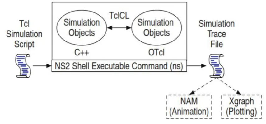
practices. Figure(1) below demonstrates the essential structural engineering of NS-2. NS-2 furnishes
clients with an executable summon ns which tackles data contention, the name of a Tcl scripting
document. Clients are putting forth the name of a Tcl recreation script as an info contention of a NS-2
executable summon ns. Much of the time, a reenactment follow document is made, and is utilized to
plot diagram and/or to make movement.
Fig (1): Architecture of NS-2
NS-2 simulation consists of two distinct phases.
Phase I: Network Configuration Phase
In this stage, NS-2 builds a system and sets up initializations. The beginning set of steps comprises of occasions
that are schedu1ed to happen at sure times (e.g., begin TFTP movement at 4 second.). This stage compares to
each 1ine in a Tcl recreation script before executing instproc run{} of the Simulator object.
Phase II: Simulation Phase
This part relates to a single line, which summons instproc Simulator::run {}. Humorously, this single line adds
to most of the recreation. In this part, NS-2 moves along the chain of events and executes every event
chain of occasions. In NS-2, "starting the event" or "terminating the event" signifies "taking activities relating to
that occasion". An activity is, for instance, beginning TFTP movement or making another occasion and
embeddings the made occasion into the chain of occasions.
The fo1lowings are the three key steps in defining a simulation scenario in a NS-2:
Step I: Simulation Design
The first step in simulating any network is to first design the simulation. In this stride, the clients ought to focus
the recreation purposes, system design and suppositions, the execution steps, and desired results.
Step II: Configuring and Running Simulation
This step implements the design. It in turn consists of two phases:
• Network configuration phase: In this phase network components (e.g., node, TCP and UDP traffic and agents)
are initialized, created and configured as per the the simulation design requirements. Also, the events such as
data transmission are scheduled to start at a stipulated time.
• Simulation Phase: his phase begins the simulation which was decided in the previous phase. It keeps the
simulation clock going and executes the various events sequentially. This stage for the most part keeps running
until the simulation clock came to an edge. By and large, it is helpful to characterize a simulation situation in a
Tcl scripting record and nourish the document as a data contention of a NS-2 syntax.
Step III: Post Simulation Processing
The important task in this step includes verifying the overall durability of the program and estimating the
accomplishment of the simulated network. While the first duty is debugging, the next one is nothing but
properly collecting and compiling the simulation results.
III. IMPLEMENTATION
The various modules in the theses are,
Network model
DSR algorithm
Received signal strength indication
Link quality indication
3.1 Network Model
Network model comprises of steps that talks about how the network environment is designed. For defining the
network various parameters have to be initialized and defined with values that suits our project requirement.
Then the simulation window has to be defined. Even that has a number of parameters to be defined. Then the
basic and the most important aspect of the project, the wireless nodes, have to be created as per the requirement.
Then the created nodes have to be deployed in the simulation environment. Required positions are assigned to
the deployed nodes. Then the nodes travel to those positions. All these processes happen in the network model
module.
3.2 DSR Algorithm
The next step is the DSR algorithm. This comes as the inbuilt functionality in NS2. We just have to mention it
as a parameter value. e have a parameter called „routing protocol‟ in NS . here we‟ll just mention as DS .
The initial process of DSR includes sending the hello packets to discover the neighboring nodes. The hello
packet originates from the first node. From there onwards the packets are broadcasted or flooded into the
network. All the neighboring nodes are discovered and the proximity of each node from every other node is
ca1cu1ated. These distances are recorded in a file as it is needed for the further steps of the project.
3.3 Received Signal Strength Indication
Once all the neighboring nodes are discovered and the distances between all the nodes are recorded, the next
step is to calculate the RSSI value for each node. RSSI is calculated at the receiver end once the packet from the
source reaches it. The value thus obtained tells us how far is the receiver from the source. Higher the RSSI
value, higher will be the signal power at the receiver and hence that node with highest recorded RSSI value is
considered to be the nearest one from the source. That is the purpose of calculating the RSSI value, to find the
nearest node for next hop, that has high signal strength for received packet. Sometimes even though a particular
node is very near, the RSSI value recorded for that node will be less because of problems like noise and jitter.
Hence our priority is the most nearest node with highest RSSI among all the available neighbors. Here we are
not sending exclusive packets just for the calculating the RSSI value. The ca1cu1ation is done depending on the
hello packets that are transmitted in the initial stage.
3.4 Link Quality Indication
As the name suggests, LQI is used to maintain the quality of the transmission link. In other words we are
making sure that the packet sent from the source reaches the intended destination in spite of adversaries like link
failures or packet loss. Once the RSSI value is calculated, based on the values thus obtained we decide the
intermediate nodes for the transmission. For each of the intermediate node, we assign two helper nodes. The
intermediate node sends election request to its immediate neighbors, which are again selected based on RSSI
values only. Two such nodes are selected for each intermediate node that has the next best RSSI value when
compared to the intermediate nodes. This election procedure has to be intimidated to the source node as well.
Packet that comes to the intermediate node is saved as a copy in the secondary helper nodes as well. In case a
then the helper nodes come into role immediately. They forward the packet on the behalf of its parent node.
Thus the retransmission request need not be sent all the way to the source node. This saves considerable
transmission time, bandwidth and energy of the nodes.
3.5 Performance Analysis
The data regarding the simulation is recorded in trace files. That data is extracted and comparison is done using
graphs. The graphs thus plotted are studied and conclusion is drafted.
WSNs are used in different scenarios. Monitoring the environment in a targeted area is more interesting in WSN
implementation, such as using wireless sensors during a forest fire to monitor the fire and its movements. The
data from sensors should be collected and then received and analyzed in the sink. In most of the scenarios, the
sinks are not in the RF range of wireless sensors, and intermediate nodes should relay the data toward the sink.
The use of a proper and efficient routing protocol affects the efficiency, reliability, and lifetime of the network.
Routing protocols use metrics to find the best path to the sink. Hop count (HC) is the most popular and is the
Internet Engineering Task Force (IETF) standard metric. It is simple to calculate, even by the devices that have
low resources in the central processing unit, memory, or energy, such as wireless sensors. This metric avoids
any computational burden on devices regarding calculation of the best route to the destination on routing
protocols. The path weights are equal to the total number of routers through it. To measure and maintain the link
quality, the protocols should send packets and use an RF module. To avoid using more energy in the RF module
for sending packets to maintain link-quality measurement, the use of RSSI or LQI is proposed in this article.
SSI is a dimensionless quantity that is measured at the receiver‟s antenna. It represents the signal strength
observed at the receiver at the moment of reception of the packet. The measurement of RSSI is not accurate due
to floor noise and current interfering transmission. We assume that WSNs are used in outdoor environments
where there is no noise or where the interference is minimal, based on the time-division technique that avoids
concurrent communication. RSSI is provided by most of the wireless sensor chips. The CC2420 chip has a
built-in RSSI that provides a digital value. The LQI is a lbuilt-ink quality metric that is measured built-in most wireless sensor
chips. CC2420 provides an LQI measurement based on the characterization of the strength and quality of a
received packet, as it is defined by IEEE 802.15.4. In this article, RSSI, and LQI have been measured in
simulation environments.
IV. RESULTS
As explained earlier, this theses was implemented in a simulation environment. The simulator used is NS-2. The
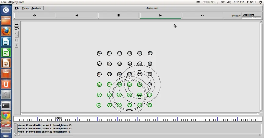
following images were taken in the form of screenshots during the process of simulation. In figure (2) we can
see that the nodes are deployed into the network. The deployed nodes have taken their respective places in the
network environment. The first step after that is to send out the hello packets to discover the neighbour nodes. It
is a necessary step in any simulation done in NS-2 which involves wireless nodes. Once that is done, in figure
(3) we can see that the nodes are broadcasting the route request packets. This is the first step in DSR algorithm
implementation. Once the destination node receives the route request packet, it sends out the route reply packets
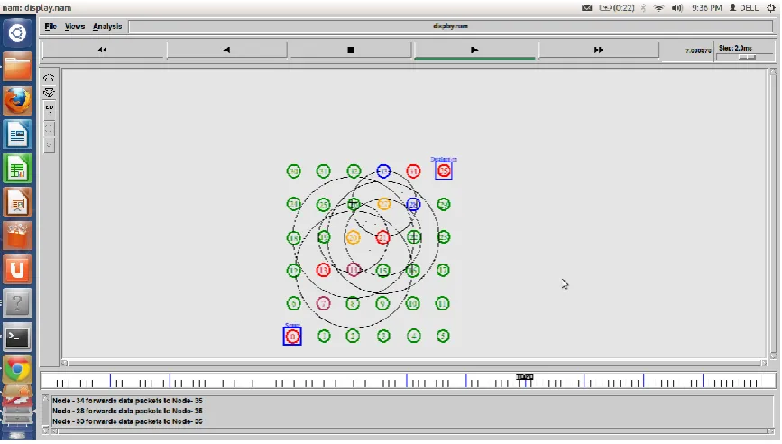
all the way to the source node. That is how the intermediate nodes are chosen. In figure (4) we can see that the
main intermediate node has to fail, at that time, these helper nodes take up the job of delivering the packet to the
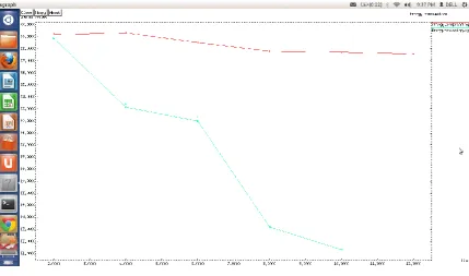
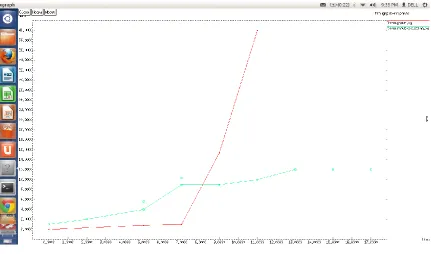
destination. The data transmission phase is seen in figure (5). Figures (6) through (8) show the results studied in
graphical form. It shows the comparison between the original DSR algorithm, and the new one with the RSSI
and LQI features added to it. The captions under the graph makes it self explanatory.
Fig (2): Nodes broadcasting hello packets for neighbour discovery.
Fig (4): Each intermediate node selects two helper nodes.
Fig (6): PDR comparison graph of proposed and existing system.
Fig (8): Throughput comparison graph of proposed and existing system.
V. CONCLUSION
In wireless sensor networks there has always been a fuss about finding the most efficient routing algorithm that
utilizes the available resources in an most efficient way possible. This project is one such effort in that front.
Here we have tried to improve the already existing routing algorithm, that has been already proved by many as
the better option when compared with rest of its peers. We took two of the performance analysis parameters and
made them to operate as routing metric. The results shown in the graphs, speak for themselves. We can see that
the proposed algorithm is showing some improved performance when compared to the existing algorithm. In
other words, here we are trying to prove, using graphical analysis, that both RSSI and LQI can be made to work
together to obtain an efficient routing metric.
This is just a small step towards a bigger picture. More such metrics can be brought together and can be
made to work as routing metrics. Each of them would provide a new advantage with additional features. DSR,
being a simple and „easy-to-understand‟ type of algorithm, provides the flexibility for such improvements.
Hence, there is always scope for further improvement of this algorithm.
In this implementation the input values are hardcoded. But they can be made to be taken as runtime
arguments. And also the node positions are also hardcoded in this implementation. Even they can be altered to
take on random positions, so that for every run of the project, the nodes assume different positions. This makes
the project more interactive and real-time. And further research can be done on more such new metrics that can
be incorporated with the existing routing algorithms to make them better than what they are right now. They
REFERENCES
Papers
“A case study of internet of things using wire ess sensor networks and smart phones,” by A. sitsigkos, F.
Entezami, T. A. Ramrekha, C. Po1itis, , pub1ished in Proc. Wire1ess Wor1d Research Forum (WWRF)
Meeting: Techno1ogies Visions Sustainab1e Wire1ess lnternet, Athens, Greece, 20l2.
“lntroduction to simu ation: lntroduction to simu ation,” by . G. lnga ls, pub ished in SC ‟ : ln the
Proceedings of the 34th conference on Winter simu1ation. Winter Simu1ation Conference, 2002.
3 “ outing protoco metrics for wire ess mesh networks,” by F. Entezami and C. Po itis, submitted at the
Wire1ess Wor1d Research Forum (WWRF) Meeting: Techno1ogies Visions Sustainab1e Wire1ess lnternet,
Ou1u, Fin1and, in Apr. 23–25, 2013.
“An enhanced routing metric for fading wire ess channe s,” by D. de O. Cunha, O. Duarte, and G. Pujo le,
pub1ished in IEEE Wireless Communications Networking Conf., 2008, pp. 2723–2728.
[5] lmp1ementation of DSR Protoco1 in NS-2 simu1ator by Venkatapathy Ragunath. University of Bonn.
[6] 1ntroduction to Network Simu1ator NS-2, by Teerawat Issariyaku1, Ekram Hossain, Springer, lst edition,
2008
7 “Load migrating for the hot spots in wire ess sensor networks using C P,” by J. Zhao, L. ang, . Yue, Z.
Qin, and M. Zhu, submitted at the 7th Int. Conf. IEEE Mobile Ad-hoc Sensor Networks, 2011.
8 “An interference and ink qua ity aware routing metric for wire ess mesh networks,” by U. Ashraf, S.
Abdel1atif, and G. Juano1e, submitted in Proc. lEEE 68th Vehicu1ar Techno1ogy Conf., 2008.
9 “An enhanced routing metric for ad hoc networks based on rea time test bed,” by F. Entezami, . A.
Ramrekha, and C. Po1itis, published in Proc. 20l2 lEEE l7th Int. Workshop Computer Aided Mode1ing Design
Communication 1inks Networks, 2012.
“Understanding packet de ivery performance in dense wire ess sensor networks.” y J. Zhao and .
Govindan. (2003). Presented at the lst lnt. Conf. Embedded Networked Sensor Systems. New York.
“Comp ex behavior at Sca e: An experimenta study of ow power wire ess sensor networks,” by D.
Ganesan, B. Krishnamachari, A. Woo, D. Cul1er, D. Estrin, and S. Wicker, presented at UCLA Computer. Sci.
Dept., Stephen Wicker Cornel1 Univ., Ithaca, NY, Tech. Rep. UCLA/CSDTR 02–0013, 2002.
“Understanding the causes of packet de ivery success and fai ure in dense wire ess sensor networks” by
K. Srinivasan, P. Dutta, A. Tavako1i, and P. Levis. (2006). Presented at the 4th lnt. Conf. Embedded Networked
Sensor Systems. New York.
3 “ SSI is under appreciated,” by K. Srinivasan and P. Levis, presented in Proc. 3rd Workshop Embedded
Networked Sensors, 2006.
“ aming the under ying cha lenges of re iable mu tihop routing in sensor networks,” by A. oo, .
Tong, and D. Cu1ler, submitted in Proc. lst Int. Conf. Embedded Networked Sensor Systems, 2003.
5 “SCALE: A tool for simp e connectivity assessment in ossy environments,” by A. Cerpa, N. usek, and
D. Estrin, presented at the Center for Embedded Networked Sensing, Univ. Ca1ifornia, Los Angeles, CA, Tech.
Rep. CCR-0120778, 2003.
6 “ e os: Enab ing u tra- ow power wire ess research,” J. Po astre, . Szewczyk, and D. Cul er,
7 “Designing a re iable and stab e ink qua ity metric for wire ess sensor networks,” by M. ondinone, J.
Ansari, J. Riihijärvi, and P. Mähönen, submitted in Proc. Workshop Rea1-Wor1d Wire1ess Sensor Networks,
2008.