Western University Western University
Scholarship@Western
Scholarship@Western
Electronic Thesis and Dissertation Repository
9-19-2011 12:00 AM
Addressing Computational Complexity of High Speed Distributed
Addressing Computational Complexity of High Speed Distributed
Circuits Using Model Order Reduction
Circuits Using Model Order Reduction
Ehsan Rasekh
The University of Western Ontario Supervisor
Dr A. Dounavis
The University of Western Ontario
Graduate Program in Electrical and Computer Engineering
A thesis submitted in partial fulfillment of the requirements for the degree in Doctor of Philosophy
© Ehsan Rasekh 2011
Follow this and additional works at: https://ir.lib.uwo.ca/etd
Part of the Computational Engineering Commons, Numerical Analysis and Scientific Computing Commons, and the VLSI and Circuits, Embedded and Hardware Systems Commons
Recommended Citation Recommended Citation
Rasekh, Ehsan, "Addressing Computational Complexity of High Speed Distributed Circuits Using Model Order Reduction" (2011). Electronic Thesis and Dissertation Repository. 267.
https://ir.lib.uwo.ca/etd/267
This Dissertation/Thesis is brought to you for free and open access by Scholarship@Western. It has been accepted for inclusion in Electronic Thesis and Dissertation Repository by an authorized administrator of
ADDRESSING COMPUTATIONAL COMPLEXITY OF HIGH SPEED DISTRIBUTED CIRCUITS USING MODEL ORDER REDUCTION
(Spine title: Numerical Reduction Techniques for Electronic Systems)
(Thesis format: Monograph)
by
Ehsan Rasekh
Graduate Program in Engineering Science Department of Electrical and Computer Engineering
A thesis submitted in partial fulfillment of the requirements for the degree of
DOCTOR OF PHILOSOPHY
The School of Graduate and Postdoctoral Studies The University of Western Ontario
London, Ontario, Canada
ii
THE UNIVERSITY OF WESTERN ONTARIO School of Graduate and Postdoctoral Studies
CERTIFICATE OF EXAMINATION
Supervisor
______________________________ Dr. A. Dounavis
Supervisory Committee
______________________________
Examiners
______________________________ Dr. K. Adamiak
______________________________ Dr. S. Asokanthan
______________________________ Dr. R. Khazaka
______________________________ Dr. J. Sabarinathan
The thesis by
Ehsan Rasekh
entitled:
Addressing Computational Complexity of High Speed Distributed Circuits
Using Model Order Reduction
is accepted in partial fulfillment of the requirements for the degree of
Doctor of Philosophy
______________________ _______________________________
iii
Abstract
Advanced in the fabrication technology of integrated circuits (ICs) over the last couple of
years has resulted in an unparalleled expansion of the functionality of microelectronic
systems. Today’s ICs feature complex deep-submicron mixed-signal designs and have found
numerous applications in industry due to their lower manufacturing costs and higher
performance levels. The tendency towards smaller feature sizes and increasing clock rates is
placing higher demands on signal integrity design by highlighting previously negligible
interconnect effects such as distortion, reflection, ringing, delay, and crosstalk. These effects
if not predicted in the early stages of the design cycle can severely degrade circuit
performance and reliability.
The objective of this thesis is to develop new model order reduction (MOR)
techniques to minimize the computational complexity of non-linear circuits and electronic
systems that have delay elements. MOR techniques provide a mechanism to generate reduced
order models from the detailed description of the original modified nodal analysis (MNA)
formulation.
The following contributions are made in this thesis:
1. The first project presents a methodology for reduction of Partial Element Equivalent
Circuit (PEEC) models. PEEC method is widely used in electromagnetic
compatibility and signal integrity problems in both the time and frequency domains.
The PEEC model with retardation has been applied to 3-D analysis but often result in
iv
a new moment matching technique based on Multi-order Arnoldi is described to
model PEEC networks with retardation.
2. The second project deals with developing an efficient model order reduction
algorithm for simulating large interconnect networks with nonlinear elements. The
proposed methodology is based on a multidimensional subspace method and uses
constraint equations to link the nonlinear elements and biasing sources to the reduced
order model. This approach significantly improves the simulation time of distributed
nonlinear systems, since additional ports are not required to link the nonlinear
elements to the reduced order model, yielding appreciable savings in the size of the
reduced order model and computational time.
3. A parameterized reduction technique for nonlinear systems is presented. The
proposed method uses multidimensional subspace and variational analysis to capture
the variances of design parameters and approximates the weakly nonlinear functions
as a Taylor series. An SVD approach is presented to address the efficiency of reduced
order model. The proposed methodology significantly improves the simulation time
of weakly nonlinear systems since the size of the reduced system is smaller than the
original system and a new reduced model is not required each time a design
parameter is changed.
Keywords
Reduced order systems, multi-order arnoldi, krylov-subspace, nonlinear systems,
interconnections, transmission lines, analog circuits, partial element equivalent circuit
v
Acknowledgments
This thesis could not be successful without the support of my supervisor Dr. Anestis
Dounavis of the Department of Electrical and Computer Engineering, University of Western
Ontario. His motivation and keen acumen in this field of research has always had a positive
effect on my work.
I would also like to extend my thanks towards every faculty member, staff member
and friend of the Department of Electrical and Computer Engineering, University of Western
Ontario for their support and help at various stages of my thesis work. I would like to
specially mention my colleagues Amir Beygi, Sourajeet Roy and Majid Ahmadloo for their
invaluable advice.
Appreciation is also extended to the following IBM researchers who provided
PowerPEEC software and valuable help used in my dissertation: Dr. Albert Ruehli and
Samuel Connor.
I would also like to thank my family for the support they provided me through my
entire life. My thanks go out to my late father Akbar, my mother Zahra, my sister Lila and
my brothers Ali, Iman and Arman as being the source of inspiration in my studies. And most
of all, I must acknowledge my lovely wife and best friend, Niloofar, without whose
encouragement and endless support, I would not have had the opportunity to complete this
Table of Contents
CERTIFICATE OF EXAMINATION ... ii
Abstract ... iii
Acknowledgments ... v
Table of Contents ... vi
List of Tables ... x
List of Figures ... xi
Abbreviations ... xiii
Chapter 1 ... 1
1 Introduction ... 1
1.1 Background and Motivation ... 1
1.2 Scope And Goals ... 6
1.3 Organization of Thesis ... 8
Chapter 2 ... 10
2 Interconnect Macromodeling and Simulation ... 10
2.1 Introduction ... 10
2.2 Interconnect Models ... 11
2.2.1 Quasi-Transverse Electromagnetic Models ... 11
2.2.2 Full Wave Models ... 13
2.3 Quasi TEM Macromodeling ... 14
vii
2.3.2 Method of Characteristics ... 17
2.4 Full-wave Macromodeling ... 21
2.4.1 The electric field integral equation (EFIE) ... 21
2.4.2 The Partial Element Equivalent Circuit ... 23
Chapter 3 ... 28
3 Simulation Techniques based on Model Order Reduction ... 28
3.1 Model Order Reduction of Linear Networks with Delay Elements ... 28
3.1.1 Description of Network Equations ... 28
3.1.2 MOR of Linear Delay Networks ... 29
3.2 Model Order Reduction of Nonlinear systems ... 34
3.2.1 Formulation of Non-linear Network Equations ... 34
3.2.2 MOR of Nonlinear Systems Based on Partitioning ... 36
3.2.3 Model Order Reduction of Weakly Nonlinear Systems ... 40
Chapter 4 ... 45
4 A Multi-Order Arnoldi Approach for Model Order Reduction of PEEC Models with Retardation ... 45
4.1 Mutli-Order Arnoldi Algorithm For PEEC Networks With Retardation ... 46
4.1.1 Computation of the Reduced Order Model ... 46
4.1.2 Moment Relationship of Reduced Order Models ... 49
4.1.3 Orthonormal Subspace of Reduced Order Models ... 51
4.2 Numerical Examples ... 54
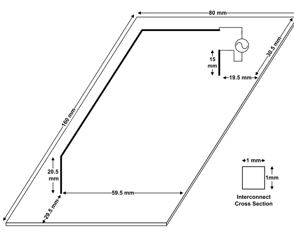
4.2.1 Example 4.1: Interconnect loop over a ground plane ... 54
viii
Chapter 5 ... 63
5 A Multidimensional Krylov Reduction Technique with Constraint Variables to Model Nonlinear Distributed Networks ... 63
5.1 Formulation of Network Equations ... 64
5.2 Nonlinear Macromodeling Using Constraint Equations ... 66
5.2.1 Formulation of Nonlinear Network Equations ... 66
5.2.2 Construction of Reduced Order Model ... 69
5.3 Implementation of Proposed Model ... 74
5.3.1 Creating a Sparse Reduced Order Macromodel ... 74
5.3.2 Selecting the Order of the Reduced Order Model ... 78
5.4 Computational Results ... 81
5.4.1 Numerical Example 5.1 ... 82
5.4.2 Numerical Example 5.2 ... 85
Chapter 6 ... 91
6 Compact Parameterized Model Order Reduction of Weakly Nonlinear System ... 91
6.1 Developing of the Parameterized Reduced Order Model ... 92
6.2 Improving the Efficiency of Reduced Order Model using SVD ... 97
6.2.1 Relationship of Moments in (6.4) ... 97
6.2.2 Terminal Reduction Framework ... 100
6.3 Computational Results ... 103
6.3.1 Example 6.1: Diode Transmission Line ... 103
6.3.2 Example 6.2: Pulse Shaping Transmission Line ... 106
ix
7 Conclusion and Future Research ... 110
7.1 Conclusion ... 110
7.2 Suggestions for Future Research ... 112
Reference ... 114
x
List of Tables
Table 4.1 CPU Run Time and Macromodel Size Comparison-Example 4.1 ... 57
Table 4.2 CPU Run Time and Macromodel Size Comparison-Example 4.2 ... 60
Table 5.1 CPU Run Time and Macromodel Size Comparison -Example 5.1. ... 84
Table 5.2 CPU Run Time and Macromodel Size Comparison- Example 5.2. ... 89
Table 6.1 CPU Run Time and Macromodel Size Comparison of Nonlinear Diode Transmission Line-Example 6.1 ... 105
xi
List of Figures
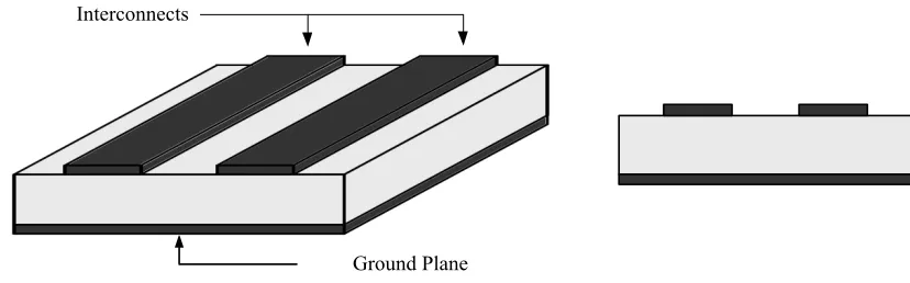
Figure 2.1 Top view and cross-sectional view of a micro-strip line network ... 11
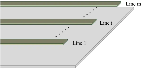
Figure 2.2 Multi-conductor Transmission Line ... 14
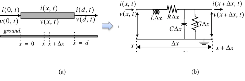
Figure 2.3 Conventional Lumped Transmission line Model. ... 17
Figure 2.4 Circuit Representation of Method of Characteristic ... 20
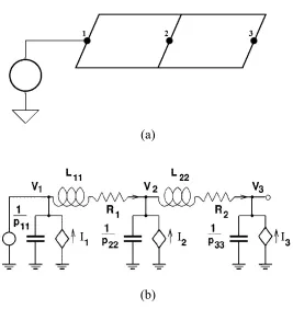
Figure 2.5 Two-conductor cell (a) and their corresponding equivalent circuit (b). ... 26
Figure 3.1 Arnoldi procedure. ... 32
Figure 3.2 Model order reduction techniques based on partitioning the network into linear and nonlinear parts. ... 37
Figure 4.1 Multi-order Arnoldi procedure. ... 48
Figure 4.2 An interconnect loop over a ground plane (Example 4.1). ... 55
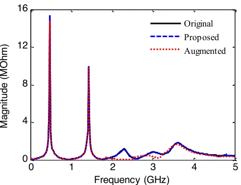
Figure 4.3 Frequency response comparison of the magnitude of the driving point impedance using one expansion point (Example 4.1). ... 56
Figure 4.4 Frequency response comparison of the magnitude of the driving point impedance using two expansion point (Example 4.1). ... 56
Figure 4.5 Three conductor wires with bend(a) layout and (b) cross-section (Example 4.2). 59 Figure 4.6 Comparison of frequency response, (a) real and (b) imaginary part of self-impedanceZab (Example 4.2). ... 61
xii
Figure 5.2 Nonlinear Distributed Interconnect Network (Example 5.1). ... 81
Figure 5.3 The transient response at node P2 for simulation of equation (5.32) (Example 5.1). ... 83
Figure 5.4 The transient response at node P2 for simulation of equation (5.33) (Example 5.1). ... 83
Figure 5.5 A coupled interconnect network with inverter terminations (Example 5.2). ... 86
Figure 5.6 Dynamic large-signal model of CMOS inverter (Example 5.2). ... 86
Figure 5.7 The transient response at nodes (a) Pout, and (b) VOUT (Example 5.2). ... 88
Figure 6.1 A nonlinear transmission line (Example 6.1). ... 103
Figure 6.2 Small signal response of nonlinear network (Example 6.1). ... 104
Figure 6.3 Small signal response of nonlinear network parameterized in capacitance (Example 6.1) ... 105
Figure 6.4 A nonlinear pulse narrowing transmission line (Example 6.2). ... 106
xiii
Abbreviations
AWE Asymptotic Waveform Evaluation.
CFH Complex Frequency Hopping.
EFIE Electrical Field Integration Equation.
EM Electromagnetic.
IC Integrated Circuit.
MNA Modified Nodal Analysis.
MGS Modified Gram Schmidt.
MOR Model Order Reduction.
MRA Matrix Rational Approximation.
ODE Ordinary Differential Equation.
PDE Partial Differential Equation.
PEEC Partial Element Equivalent Circuit.
p.u.l. Per-unit-length.
RF Radio Frequency.
SVD Singular Value Decomposition.
TEM Transverse Electromagnetic.
1
Chapter 1
1
Introductio
n
1.1
Bac
kground and Motivation
Advances in integrated circuit (IC) technology has increased operating speeds, packing
density, system complexity of electronic devices and are placing significant demands on
computer-aided design tools to provide the same efficiency and accuracy. The simulation
and verification of mixed signal ICs pose a particular problem for time domain circuit
simulators, which are based on implicit numerical integration methods that require
solving a large set of nonlinear algebraic equations at each discrete time point. As a
result, simulating the transient behaviour of ICs is arduous and computationally
expensive task. This problem is further compounded when one considers the typical
Chapter 1: Introduction 2
processes require conducting a large number of repeated simulations of the same problem
with different parameter values. At the same time shrinking process technologies
generate a need to consider low-level physical effects such as parasitic effects,
transistor-level effects, details of implementation, and signal integrity. Consequently, simple
heuristic models may not be sufficient for computational prototyping of modern
integrated circuits.
The rapid decrease in feature size and associated growth in circuit complexity,
coupled with higher operating speeds, has made the analysis of interconnects a critical
aspect of system reliability, speed of operation, and cost. As a result of these
technological advancements, Electromagnetic (EM) analysis [1]- [2] has become
essential in the design of high-speed integrated circuits. Among EM analysis techniques,
the Partial Element Equivalent Circuit (PEEC) [3]- [4] method is often used to model
complex three-dimensional interconnect and packaging structures since it can provide full
wave and quasi-static circuit equivalent models which can be linked to traditional circuit
simulators such as SPICE [5]. However, distributed interconnects and packaging
problems modeled using PEEC result in large dense system matrices, simulation of which
is computationally expensive.
Over the past years, model order reduction techniques have been proposed as an
Chapter 1: Introduction 3
they provide a mechanism to generate reduced order models from detailed descriptions
[6]- [23]. MOR techniques such as asymptotic waveform evaluation (AWE) [9]- [12],
complex frequency hopping (CFH) [13], Padé [14], Arnoldi [15]- [21], and truncated
balance reduction [22]- [23] have proven to be efficient means to reduce large linear
interconnect networks. Recently, model order reduction techniques have been extended to
model PEEC networks [24]- [32].
Model order reduction techniques applied to PEEC models can be broadly
classified into two main categories: approaches that use explicit moment matching based
on direct Padé approximants [24]- [27] and approaches that use implicit moment
matching based on projecting large matrices on its dominant eigenspace [28]- [32].
Explicit moment matching techniques such as Asymptotic Waveform Evaluation (AWE)
have been proposed to solve both quasi-static PEEC models [24]- [25] and full-wave
PEEC models that include retardation effects [26]. However, these techniques are
inherently ill-conditioned in the moment generating process and hence the reduced order
model obtained is limited to low order approximations [7]- [8]. To improve the accuracy
of AWE, Complex Frequency Hopping (CFH) has been proposed which makes use of
multiple expansion points to derive higher order transfer functions [27].
Alternatively, implicit moment matching techniques such as Krylov subspace
Chapter 1: Introduction 4
models [28]- [32]. However, the traditional Arnoldi algorithm requires that the system
equations have a linear dependency with respect to frequency. For PEEC models that
include retardation effects, the transfer function contains elements with factors of !!!!!
where !! corresponds to a time delay (retardation) in the circuit. As a result, PEEC
models with retardation are not directly compatible with the traditional Arnoldi algorithm
since they contain many delay elements. To include retardation effects using Arnoldi,
each exponential function of !!!!! is expanded into a Taylor series and the polynomial
equations are converted to have a linear dependency with respect to frequency by
introducing extra state variables [31]- [32]. Conversely, this changes the structure of the
reduced order system when compared to the original system and the extra state variables
increases the computation and memory requirements to derive the reduced order model.
Furthermore, model order reduction approach has been extended for nonlinear
circuit simulation problems [10], [19]- [20], [33]- [41]. A common strategy for
simulating distributed interconnect networks is based on partitioning the network into
linear and nonlinear parts [10], [19]- [20]. The linear network is then reduced using
moment matching techniques to form a compact multi-port time-domain macromodel.
This macromodel is then coupled with the nonlinear part of the network to obtain the
overall network response. However, the efficiency of these techniques drops significantly
Chapter 1: Introduction 5
terminations. This drop in efficiency is attributed to the fact that the size of the linear
macromodel increases by q for each additional port, where q is the size of the reduced
order macromodel with one port.
An alternative approach for model order reduction of nonlinear systems is to
directly reduce the entire nonlinear distributed network (without partitioning the linear
and nonlinear components) based on power series or piecewise polynomial
approximations. Several model order reduction techniques have been proposed to reduce
the computational complexity of nonlinear systems [34]- [41]. The reduction of weakly
nonlinear systems has been demonstrated based on power series approximations [34]-
[37]. For strongly nonlinear systems techniques based on trajectory piecewise
polynomials have been reported [38]- [41]. While these algorithms provide significant
CPU cost advantage when computing the transient response, a new reduced model is
required each time a parameter is modified in the studied structure. Recently, parametric
model order reduction techniques have been developed for linear systems, which produce
reduced order models that are functions of frequency or time as well as other design
parameters [42]- [47]. Nonetheless, these parametric models are not directly applicable to
nonlinear systems. In [48], a parametric reduced order model for nonlinear systems is
Chapter 1: Introduction 6
1.2
Scope And Goals
The objective of this thesis is to develop efficient modeling techniques for high speed
integrated circuit simulation. The focus of this research is based on model order reduction
techniques to improve the computational complexity of PEEC structures with retardation
and nonlinear distributed networks.
Distributed interconnects and packaging problems modeled using Partial
Element Equivalent Circuit (PEEC) method results in large dense system matrices,
simulation of which is computationally expensive. To include retardation effects using
Arnoldi model order reduction methods, each exponential function of !!!!! is expanded
into a Taylor series and the polynomial equations are converted to a linear form by
introducing extra state variables [31]- [32]. This changes the structure of the reduced
order system when compared to the original system and the extra state variables increases
the computation and memory requirements to derive the reduced order model.
Techniques to improve the conditioning of the moment generating process of networks
described by higher order polynomials have also been developed based on second order
Arnoldi [49]- [51], multi-order Arnoldi [52]- [54] and well-conditioned AWE [55]. In
this thesis, a multi-order Arnoldi algorithm will be developed to efficiently solve PEEC
models with retardation. The advantages of the proposed approach when compared to
Chapter 1: Introduction 7
are calculated implicitly without having to introduce extra state variables and the
structure of the reduced model is the same as the original system. Furthermore, it is
shown that the orthonormal subspace of the system built by introducing extra state
variables [31]- [32] is embedded in subspace built by the multi-order Arnoldi approach.
Partitioning the network into linear and nonlinear parts has been proposed for
addressing complexity of nonlinear distributed interconnect networks [19]- [20].
However, the efficiency of these techniques drops significantly as the number of ports of
the linear sub-network increases due to having many nonlinear terminations. In this
thesis, a model order reduction algorithm will be developed to efficiently link nonlinear
elements to the reduced order system without having to increase the number of ports. The
proposed methodology uses a multidimensional Krylov subspace method and constraint
variable equations to capture the variances of nonlinear functions and to link nonlinear
functions to the reduced order macromodel. This approach significantly improves the
simulation time of distributed nonlinear systems since additional ports are not required to
link the nonlinear elements to the reduced order model. In addition, an approach is
developed for generating sparse matrices and to select the order of the reduced order
model.
The reduction of weakly nonlinear systems has been demonstrated based on
Chapter 1: Introduction 8
cost advantage when computing the transient response, a new reduced model is required
each time a parameter is modified in the studied structure. Parameterized model order
reduction techniques will be extended for weakly nonlinear systems in this research. The
proposed algorithm uses a multidimensional subspace method along with variational
analysis and Singular Value Decomposition (SVD) to capture the variances of design
parameters and approximates the weakly nonlinear functions as a Taylor series. Such an
approach is significantly more CPU efficient in optimization and design space
exploration problems since a new reduced model is not required each time a design
parameter is modified.
1.3
Organization of Thesis
The organization of the thesis is as follows. A brief review of high-speed interconnects,
including quasi-TEM and full-wave formulations are provided in chapter 2. Full-wave
analysis of complex three-dimensional interconnects using Partial Element Equivalent
Circuit (PEEC) method is presented later in the same chapter. A review of various MOR
techniques to model PEEC networks with retardation and nonlinear distributed networks
are discussed in chapter 3. In addition model order reduction techniques of weakly
nonlinear systems is also reviewed. Chapter 4 describes the details of a multi-order
Chapter 1: Introduction 9
Numerical examples of PEEC models with retardation are provided to illustrate the
validity of the proposed technique. In chapter 5, a model order reduction algorithm using
constraint variables is developed to efficiently link nonlinear elements to the reduced
order system without having to increase the number of ports. In addition, an approach is
developed for generating sparse matrices and to select the order of the reduced order
model. Numerical examples are presented to demonstrate the efficiency of the proposed
algorithm. Parameterized model order reduction techniques are extended for weakly
nonlinear systems employing multidimensional subspace method, variational analysis
and SVD in chapter 6. This chapter concludes presenting some numerical examples to
show the efficiency of the algorithm. Chapter 7 presents a summary and suggestions for
10
Chapter 2
2
Interconnect
Macromodeling
and Simulation
2.1
Introduction
Interconnects are conducting structures that are used to connect transistors and other
devices on Integrated Circuits (IC). The physical structure of a micro-strip line
interconnect network consisting of two conductors and ground plane is shown in Figure
2.1. As frequency increases, interconnects gradually display resistive, capacitive and
inductive effects and cannot be considered as short circuit anymore. Improper
consideration of these effects can harshly degrade the signal integrity analysis of the
networks. As a result circuit designers must consider these effects to ensure the signal
integrity and proper operation of devices. In this chapter, interconnect models are briefly
Chapter 2: Interconnect Macromodeling and Simulation 11
Figure 2.1 Top view and cross-sectional view of a micro-strip line network
2.2
Interconnect Models
Electrical models are employed to simulate interconnects along with other circuit
elements in the network. The selection of the proper model depends on the physical
interconnect structure as well as the operating frequency of the circuit [56], [57]. These
two factors determine whether the modeling of interconnects is based on quasi-transverse
electromagnetic (quasi-TEM) or full wave assumptions. These two methods are described
in the following sections.
2.2.1
Quasi
-
Transverse Electromagnetic Models
Transverse electromagnetic (TEM) waves occur for interconnects with homogeneous
mediums and perfect conductors. Under these conditions electric and magnetic fields are
Interconnects
Chapter 2: Interconnect Macromodeling and Simulation 12
perpendicular to each other and to the direction of propagation in TEM waves. Structures
with imperfect conductor or inhomogeneous medium violate the TEM characteristics.
Interconnects with inhomogeneous mediums produce electromagnetic waves with many
velocities. Interconnects that have imperfect conductors also produce an electric field
along the surface conductor. Such structures violate the TEM characteristics, since TEM
waves propagate with only one velocity and have no electric field along the surface
conductor. However, for many practical structures, the electromagnetic field structure can
be approximated by TEM waves, which are referred to as quasi-TEM waves [56].
Quasi-TEM approximation remains the main trend for analyzing lossy MTLs,
since the approximation is valid for most practical interconnect structures and offers
relative low CPU cost compared to full wave approaches [56], [58]. Voltage and current
equations derived from quasi-TEM models are described by partial differential equations
(PDEs) widely known as Telegrapher's equations. As frequency increases proximity,
edge, and skin effects become prominent and distributed models with
frequency-dependent parameters are required. Quasi-TEM distributed models cannot be directly
linked to circuit simulator such as SPICE [5], since SPICE solves nonlinear ordinary
differential equations (ODEs). To overcome this difficulty, numerical techniques are used
to convert distributed transmission line models into ODEs.
Chapter 2: Interconnect Macromodeling and Simulation 13
linking distributed transmission lines to circuit simulators. Electrical length of the
transmission line determines the number of segments required for modeling. For
transmission lines that the length of the line is much greater than the wavelength many
segments are required for proper modeling. In addition to the lumped segmentation
model, other more sophisticated algorithms exist such as the method of characteristics
[59]- [63], Chebyshev polynomials [64]- [65], wavelets [66]- [67], Matrix Rational
Approximation (MRA) [68] and congruent transformation [69].
2.2.2
Full Wave Models
If the cross-sectional dimensions of interconnects become a significant fraction of the
circuit's operating wavelength, the field components in the direction of propagation can
no longer be ignored [56] and quasi-TEM assumptions become inadequate in describing
interconnects. Under these conditions, full wave models are required. These models are
able to account for all possible field components and satisfy all boundary conditions
required to accurately model the high-frequency effects of interconnect networks.
Full wave analysis of interconnect structures have been successfully
implemented using partial element equivalent circuit (PEEC) models [3]- [4]. PEEC
models including retardation effects provide a full wave solution. Regular PEEC models
Chapter 2: Interconnect Macromodeling and Simulation 14
Figure 2.2 Multi-conductor Transmission Line
static solution of Maxwell's equations. These models usually produce large and dense
circuit networks and are very CPU intensive to solve.
2.3
Quasi TEM
Macromodeling
In this section, methods for quasi-TEM analysis of transmission lines are presented.
Consider a lossy coupled interconnect network containing m signal conductors and one
reference conductor as shown in Figure 2.2. The voltages and currents are functions of
position x, and time t and can be defined as vectors v(x,t) and i(x,t)∈ℜ!. Considering
quasi-TEM distributed assumptions, voltages and currents are related by Telegrapher's
equations [56] as
Line 1
Line i
Chapter 2: Interconnect Macromodeling and Simulation 15
!
!xv(x,t)="Ri(x,t)"L ! !ti(x,t) !
!xi(x,t)="Gv(x,t)"C ! !tv(x,t)
(2.1)
where R∈ ℜ!×!, L ∈ℜ!×!, G ∈ℜ!×!, C ∈ℜ!×! are per unit length (p.u.l.)
resistance, inductance, conductance and capacitance of the multi-conductor transmission
line, respectively.
To simulate interconnects with other linear and nonlinear elements,
macromodels are required to convert Telegrapher’s equations into ODEs which can be
solved by commercial circuit simulators. Determining the frequency bandwidth of
interest is an important issue in constructing macromodels. In digital applications, the
frequency bandwidth of interest is governed by the rise/fall time of the signal. For
instance, consider a trapezoidal pulse with an energy spectrum spread over an infinite
frequency range, main part of the signal energy is concentrated in the low frequency
region and eliminates rapidly with an increment in frequency [11]. Hence, disregarding
the high-frequency component of the frequency spectrum above a maximum frequency of
interest will not effect the overall signal shape. Relationship between the maximum
frequency of interest fmaxand the rise/fall time of the trapezoidal pulse tr is determined
Chapter 2: Interconnect Macromodeling and Simulation 16
fmax !k/tr (2.2)
where k typically ranges from 0.35 to 1 [11], [70]- [71].
The next sections review some of the simulation algorithms that are used for
Quasi-TEM macromodeling of transmission lines.
2.3.1
Conventional Lumped
Method
This method uses lumped equivalent circuits to approximate Telegrapher’s Equation
(2.1). Applying Euler’s method [56] to discretize (2.1) yields
v(x+!x,t)"v(x,t)="!xRi(x,t)" !xL # #ti(x,t)
i(x+!x,t)"i(x,t)="!xGv(x+!x,t)" !xC #
#tv(x+!x,t)
(2.3)
where Δx=d/M is the length of each section, d is the length of transmission line and M is
the number of needed segments. A circuit representation of equation (2.3) is shown in
Figure 2.3.
The conventional lumped model provides a direct discretization method for
interconnects; however, the model is only valid if Δx is chosen to be a small fraction of
Chapter 2: Interconnect Macromodeling and Simulation 17
(a) (b)
Figure 2.3 Conventional Lumped Transmission line Model.
electrically long many lumped elements are required. A rule of thumb for selecting the
number of sections in Hspice [72] is
M = 20 LC d
tr
(2.4)
As the length of the line and as operating frequency increases many lumped sections are
required to accurately capture the signal. This leads to large circuit matrices, making the
method inefficient.
2.3.2
Method of Characteristics
The method of characteristics [59] represents lossless interconnects as ODEs containing
22
riously effect the overall signal shape. A useful relationship between the maximum frequency of interest ( ) and the rise/fall time of the signal ( ) is
(2.39)
which corresponds to the 3-dB bandwidth point of the energy spectrum [7], [19], [74]. For high-frequency applications, the maximum frequency can be more conservatively set to [7],
(2.40)
The following sections review some of the simulation algorithms that are used for mac-romodeling transmission lines.
2.5.1 Conventional Lumped Segmentation
This method uses lumped equivalent circuits to approximate (2.2). Applying Euler’s method [2] to discretize (2.2) yields
(2.41)
where is the length of each section, dis the length of the total line and Mis the number of segments. A circuit representation of equation (2.41) is shown in Figure 2.7.
fmax tr
fmax!0.35⁄tr
fmax!1⁄tr
v(x x+ ",t)–v(x t, ) –"xRi(x t, ) "xL
t
##i(x t, )
– =
i(x+"x t, )–i(x t, ) = –"xGv(x+"x t, )–"xC##tv(x+"x t, )
"x = d M⁄
Figure 2.7 Lumped transmission line model i x t( , )
i(0,t)
v x t( , )
v(0,t)
i d t( , ) v d t( , )
x = 0 x x = d
ground
R"x L"x
C"x G"x i x t( , )
v x t( , )
i x( +"x,t) v x( +"x,t)
"x x
x+"x
(a) (b) x+"x
22
riously effect the overall signal shape. A useful relationship between the maximum frequency of interest ( ) and the rise/fall time of the signal ( ) is
(2.39)
which corresponds to the 3-dB bandwidth point of the energy spectrum [7], [19], [74]. For high-frequency applications, the maximum frequency can be more conservatively set to [7],
(2.40)
The following sections review some of the simulation algorithms that are used for mac-romodeling transmission lines.
2.5.1 Conventional Lumped Segmentation
This method uses lumped equivalent circuits to approximate (2.2). Applying Euler’s method [2] to discretize (2.2) yields
(2.41)
where is the length of each section,dis the length of the total line andMis the number of segments. A circuit representation of equation (2.41) is shown in Figure 2.7.
fmax tr
fmax!0.35⁄tr
fmax!1⁄tr
v(x x+ ",t)–v(x t, ) = –"xRi(x t, )–"xL##ti(x t, )
i(x+"x t, )–i(x t, ) –"xGv(x+"x t, ) "xC
t
##v(x+"x t, )
– =
"x = d M⁄
Figure 2.7 Lumped transmission line model
i x t( , )
i(0,t)
v x t( , ) v(0,t)
i d t( , ) v d t( , )
x = 0 x x = d
ground
R"x L"x
C"x G"x i x t( , )
v x t( , )
i x( +"x,t) v x( +"x,t)
"x x
x+"x
Chapter 2: Interconnect Macromodeling and Simulation 18
time delays. Method of characteristics was initially developed in the time-domain using
what is referred as characteristic curves. A simpler alternative derivation in the
frequency-domain is presented in this section. The Laplace domain solution of (2.1) for
two-conductor transmission line [73] is
I1 I2 ! " # # $ % & &= 1
Z0
(
1'e'2!d)
1+e'2!d
2e'!d
'2e'!d
1+e'2!d
! " # # $ % & & V1 V2 ! " # # $ % & & (2.5) where
! = (R+sL)(G+sC) Z0 =
(R+sL)
(G+sC) (2.6)
! is the propagation constant and !! is the characteristic impedance. The terms in (2.5)
can be re-formulated to
V1=Z0I1+e
!!d
2V2!e
!!d
(Z0I1+V1)
"# $%
V2 =Z0I2+e
!!d
2V1!e
!!d
(Z0I2+V2)
"# $% (2.7)
Chapter 2: Interconnect Macromodeling and Simulation 19
W1=e!!d
2V2!e!!d
(Z0I1+V1)
"# $%
W2 =e
!!d
2V1!e
!!d
(Z0I2+V2)
"# $%
(2.8)
and substituting (2.8) in (2.7) yields
V1=Z0I1+W1
V2 =Z0I2+W2
(2.9)
Eliminating the terms !!!! and !!!! in (2.8) using (2.9) results in
W1=e
!!d
2V2!e
!!d
(2V1!W1)
"# $%
W2 =e
!!d
2V1!e
!!d
(2V2!W2)
"# $% (2.10)
Considering the symmetry of (2.10) the following recursive relationship for W1 and W2 is
obtained
W1 =e
!!d
2V2!W2
[
]
W2 =e
!!d
2V1!W1
[
]
(2.11)Chapter 2: Interconnect Macromodeling and Simulation 20
Figure 2.4 Circuit Representation of Method of Characteristic
! =s LC Z0 = L
C (2.12)
This restriction makes propagation constant ! purely imaginary and characteristic
impedance !! a real constant. The time-domain representation of (2.11) is obtained by
taking the Laplace inverse, which replaces !!!"by delays, expressed as
w1(t+!)=2v2(t)!w2(t)
w2(t+!)=2v1(t)!w1(t)
(2.13)
A circuit representation of the transmission line modeled using method of characteristics
is shown in Figure 2.4. For the case of lossy lines, propagation constant ! is not purely
imaginary and characteristic impedance !! is not a real constant, hence (2.10) cannot be
directly expressed in time-domain. In order to model lossy transmission lines, the method
of characteristics approximates the losses of propagation constant and characteristic
25
2.5.3 Least Square Optimization
Least square optimization techniques [27] derive transfer functions for the frequency re-sponse of transmission lines. The method fits sample data to a complex rational function as
(2.50)
where , and represent the quotient, residues and poles, respectively. To obtain sta-ble poles, the even part ofH(s)is fitted to the real data samples. The even part ofH(s) is expressed as
(2.51)
where and is the angular frequency. Writing (2.51) at the frequency points , yields the following set of linear equations
(2.52) Z0 + – w1 Z0 +
– w2
v1 v2
+ +
– –
Figure 2.8 Method of characteristics transmission line model.
i2 i1
H s( ) c ki s p– i ---i=1
N
!
+ =c ki pi
Re H s( ( ))
ai( )"2 i
i=0
N
!
1 bi( )"2 i
i=1
N
!
+---=
s = j" " "0,"1, ,… "K
[ ]
1 "02 … "02N –"02Re H( ( )"0 ) … –"02NRe H( ( )"0 )
1 "12 … "12N –"12Re H( ( )"1 ) … –"12NRe H( ( )"1 )
1 "2K … "K2N –"2KRe H( ("K)) … –"K2NRe H( ("K))
a0
aN b1
bN
Re H( ( )"0 ) Re H( ( )"1 )
Re H( ("K))
=
}
Chapter 2: Interconnect Macromodeling and Simulation 21
impedance as rational functions [60]- [61], [74]- [75]. In addition, the method of
characteristics has been extended to multi-conductor transmission lines, by decoupling of
the transmission line equations [62]- [63], [76].
2.4
Full
-
wave Macromodeling
In this section, the derivation of the electric field integral equation (EFIE) is described.
From this discussion the Partial Element Equivalent Circuit (PEEC) macromodel is
derived as a system of ordinary delay-differential equation.
2.4.1
The electric field integral equation (EFIE)
The total electric field inside a conductor is given by [77]
Ep
( )
r,t =J r
( )
,t! +
!A r
( )
,t!t + "!
( )
r,t (2.14)where Ep is a potential applied electric field, J is a current density, A is the magnetic
vector potential, and ! is the scalar electric potential. The vector potential A of a single
Chapter 2: Interconnect Macromodeling and Simulation 22
A r
( )
,t =µ G( )
r,r! J(
r!,td)
dv!! v
"
(2.15)where !′ is the volume of material in which the current density is flowing and µ is the
permeability of free space. The retarded time !! is given by
td =t!
r! "r
c (2.16)
where c is the speed of light. The time delay equals the free space travel time between the
points ! and !′. The corresponding Green’s function is given by
G
( )
r,r! " 14! 1
r# !r (2.17)
Similarly, the scalar potential
!
( )
r,t = 1"0
G
( )
r,r! q(
r!,td)
dv!! v
"
(2.18)where !! is the dielectric constant in free space, and q is the charge density on the
surface. Assuming external electric field is zero and substituting (2.15) and (2.18) into
Chapter 2: Interconnect Macromodeling and Simulation 23
J r
( )
,t! +µ G
( )
r,r!"J
(
r!,td)
"t dv!!
v
#
+ $!0
G
( )
r,r! q(
r!,td)
dv!! v
#
=0 (2.19)2.4.2
The Partial Element Equ
ivalent C
ircuit
Particular spatial discretization of the conductor geometry combined with the integral
equation (2.19), lead to Partial Element Equivalent Circuit (PEEC) models with
conventional circuit elements. By defining a suitable inner product, a weighted volume
integral over the cells, the field equation (2.19) can be interpreted as Kirchhoff’s voltage
law over a PEEC cell. This is accomplished by the breakup of the geometry into 2-D or
3-D cells, the integration of (2.19) over each resulting conductor volume cell [3], and
observing that the first term in (2.19) corresponds to a resistor, the second term can be
transformed into partial inductances [78], and the last term corresponds to normalized
coefficients of potential [79]. The partial inductances are defined as
Lij
( )
s =µ
aiaj
G
( )
ri, rj e!std
dvidvj
vi
"
v
"
j(2.20)
where !! and !! correspond to through the cell cross section of partial elements. The
Chapter 2: Interconnect Macromodeling and Simulation 24
(2.21)
where !! and !!are cell areas. By using (2.20) and (2.21), the discredited EFIE (2.19) is
reformulated in the form of [3]:
sL(s)I!BP(s)Q(s)+RI(s)=0
BT
I(s)+sQ(s)=0
(2.22)
where B contains the connectivity information of the discretization and
L(s)= Lke
!stdk k=0
n1
"
P(s)= Pke
!stdk k=0
n2
"
(2.23)
!! and !! are number of delay terms of the coefficients of partial inductance and
potential coefficients. L(s) and P(s) in (2.23) contain all partial inductance and potential
coefficients respectively. Matrix elements in R, Q and I are defined by the following
equations
Pij
( )
s = 1!0SiSj G
( )
ri,rj e!stdds
idsj si
"
sjChapter 2: Interconnect Macromodeling and Simulation 25
Rii= li
ai!
Qi(s)= qi
( )
r!,s dv!! v
"
Ii(s)= Ji
( )
r,s dsa
"
(2.24)
which are resistance, charge and current passing the ith cell, respectively
The system in (2.22) can be interpreted as an electronic circuit, where each circuit
node represents a charge basis function and each current basis function is represented by
circuit branch. The coefficients of potential are related to the electrostatic potential with
V=PQ. The electrostatic potential at the charge segments will be the nodal voltages in the
circuit. The charge accumulation on the charge segments is written as an extra set I=sQ .
Substituting these two definitions in (2.22) yields [3]
sL
( )
s I!BV+RI=0BT
I+Is =0
P
( )
s Is!sV=0(a)
(b)
(c)
(2.25)
In this formulation, a set of branch constitutive relations for branches with a linear
resistor, and an inductor that couples to all other inductors in (2.25.a), in series can be
Chapter 2: Interconnect Macromodeling and Simulation 26
(a)
(b)
Figure 2.5 Two-conductor cell (a) and their corresponding equivalent circuit (b).
is discerned. The third one, (2.25.c), can be interpreted as a set of branch constitutive
relations for coupled capacitances. These capacitances store the charge that is
accumulated on the charge segments. For PEEC models with retardation, the
corresponding Modified Nodal Analysis (MNA) equations reduce to systems of linear,
time-invariant, delay-differential-algebraic equations. After adding the relationship
Chapter 2: Interconnect Macromodeling and Simulation 27
system is obtained
sC0+G0+
(
sCk+Gk)
e!stdk
k=0 nT
"
# $%
&
'(X(s)=Bu(s)
i(s)=LT X(s)
(2.26)
where !! is the total number of exponentials which corresponds to the number of time
delays !!" of the system. The matrices Gk, Ck ∈ℜ!×! correspond respectively to the
state and to the derivative of the state. !(!) ∈ℂ! is a vector of the unknown state
variables. The matrices B ∈ℜ!×! and L∈ℜ!×! are selector matrices which map the
terminal port characteristics; k is the number of ports; u(s), i(s) ∈ℂ! define the port
voltages and currents of the network, respectively and N is the number of unknown
variables in X(s). A schematic of a simple two-cell PEEC model is given in Figure 2.5.
The discretization of two cells is shown in Figure 2.5(a) and Figure 2.5(b) shows
28
Chapter 3
3
Simulation Techniques based on Model Order
Reduction
This chapter reviews Model Order Reduction (MOR) techniques used to model PEEC
networks and nonlinear distributed interconnect networks.
3.1
Model Order Reduction of Linear Networks with
Delay Elements
3.1.1
Description of Network Equations
As illustrated in section 2.4, a linear network characterized by PEEC models with
Chapter 3: Simulation Techniques based on Model Order Reduction 29
sC0+G0+
(
sCk+Gk)
e !stdkk=0 nT
"
# $%
&
'(X(s)=Bu(s)
i(s)=LTX(s)
(3.1)
In general, distributed electrical networks characterized by PEEC models with retardation
result in a very large system matrices which are dense and computationally expensive to
solve. The next section briefly reviews model order reduction techniques which reduce
the computational complexity of PEEC networks with retardation.
3.1.2
MOR of Linear Delay Networks
One approach to obtain a reduced order model for (3.1) is to explicitly calculate the
moments and to use algorithms such as Modified Gram-Schmidt to construct the
orthogonal subspace [80]. However as the number of moments increase, this leads to
numerical difficulties since the higher order moments converge to the largest eigenvalue
of the system and are almost identical or parallel to each other. To obtain numerically
more accurate results, implicit moment matching techniques such as Arnoldi algorithm
are usually preferred since they avoid explicit calculation of the moments [7], [81].
However, the original Arnoldi algorithm is only applicable for systems that have a linear
Chapter 3: Simulation Techniques based on Model Order Reduction 30
the moments using Arnoldi, the exponential terms of (3.1) are expanded into a
polynomial series as
e!tds "e!tds0 (!td)
i
i! (s!s0) i i=0
M
#
$ %& ' () (3.2)where !! is the expansion point and M is the order of the polynomial. Substituting (3.2)
into (3.1), and matching coefficients of similar powers of (s!s0) yields
!i(s"s0) i i=0
M
#
$ %&
'
()X(s)=Bu(s) (3.3)
where
!i=
G0+s0C0+
(
s0Ck+Gk)
e"s0tdk
k=1
nT
#
, i=0C0+ Cke
"s0tdk k=1
nT
#
+(
s0Ck+Gk)
e"s0tdk
k=1
nT
#
("tdk), i=1Cke"s0tdk k=1
nT
#
("tdk) i"1(i - 1)! +
(
s0Ck+Gk)
e"s0tdk
k=1
nT
#
("tdk) ii! , i$2
Chapter 3: Simulation Techniques based on Model Order Reduction 31
Once the network is expressed as a polynomial series, the system of (3.3) is
augmented to obtain a linear dependency with respect to frequency [31]- [32], [82]
as
!
G+(s!s0)C!
(
)
X! =Bu! (3.5)where
!
C=
!1 !2 !3 !4 ... !M
"I 0 0 0 ... 0
0 "I 0 0 ... 0
: :
0 0 0
# $ % % % % % % % & ' ( ( ( ( ( ( ( ; (3.6)
and I is identity matrix. The moments of (3.5) at the expansion point !! are calculated
using the following recursive relationship
!
G=
!0 0 0 0 ... 0
0 I 0 0 ... 0
0 0 I 0 ... 0
: :
0 0 I
" # $ $ $ $ $ $ $ % & ' ' ' ' ' ' ' ! X= X z2 z3 : : zM ! " # # # # # # # # $ % & & & & & & & &
;B! =
Chapter 3: Simulation Techniques based on Model Order Reduction 32
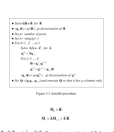
● SolveG!R =! B! for R!
● (q0,K)=qr(R!); qr factorization of R!
● Set p= number of ports
● Set n= int(q/p)+1
● For k=l , 2, …,n-1
Solve GA =! !C! for A!
q(0)k =Aq!
k!1
For j=1,…, k
H=qk!j T q
k
(j!1)
qk(j)=q k (j!1)!q
k!jH (qk,K)=qr(qk
k
( )); qr factorization of
● Set Q=[q0q1...qn!1]and truncate Q so that it has q columns only.
Figure 3.1 Arnoldi procedure.
!
M0 =R!
!
Mi =A!M! i!1=A!i! R
(3.7)
where R! =G!!1B! and A! =!G!!1C! . The matrix generated using (3.7) forms a Krylov
subspace.
!
K=!"M! 0M!1M! 2....M! n#$
= R! A!R! A!2R!....A!n !
R
!" #$
(3.8)
) (k k
Chapter 3: Simulation Techniques based on Model Order Reduction 33
Hence, the Arnoldi algorithm, as shown in Figure 3.1, can be used to convert (3.8) into an
orthonormal matrix Q! [7], [80]- [81], such that the column space of K! matches the
column space of Q! as
colsp(Q!)=colsp(K!)
!
QT!
Q=I
(3.9)
Using (3.9), the augmented system of (3.5) is reduced by a congruent transformation,
(3.10)
where
ˆ
Ga =Q!
T !
GQ!, Cˆa =Q! T!
CQ!
ˆ
Ba =Q! T!
B, X! =Q!Xˆa
(3.11)
In [31]- [32], the system of (3.10) is used to efficiently express the transfer function of
PEEC networks in terms of poles and residues. However, this approach requires
introducing M!N state variables to convert the polynomial series of (3.3) into a
first-order system. This changes the structure of the reduced first-order system when compared to
the original system and the extra state variables increase the computation and memory
Chapter 3: Simulation Techniques based on Model Order Reduction 34
requirements to derive the reduced order model by O(N2M) [31]. In [82] a projection
matrix is built using first M row of (3.8) to reduce the model in (3.1). This approach is
able to preserve the structure of the reduced order system when compared to the original
system. However, the block resulted by considering first M rows of (3.8) is not
orthogonal and therefore another round of orthogonalization has to be carried out.
Furthermore, the extra state variables increase the computation and memory requirements
to derive the reduced order model.
To address the above concerns, a multi-order Arnoldi algorithm is developed for
PEEC circuits with retardation in chapter 4. The advantages of this approach are that the
moments of the original system are calculated implicitly without having to introduce
extra state variables and the structure of the reduced model is the same as the original
system.
3.2
Model Order Reduction of
Nonlinear systems
3.2.1
Formulation of
Non
-linear
Network Equations
Consider a general nonlinear network comprised of lumped and distributed interconnects.
After discretizing the distributed components with lumped elements [56], the Modified
Chapter 3: Simulation Techniques based on Model Order Reduction 35
Cdx(t)
dt +Gx(t)+f(x(t),t)=Bu(t)
i(t)=LT x(t)
(3.12)
where
• x(t)∈ℜ! is a vector of node voltage waveforms appended by independent voltage
source currents, linear inductor currents nonlinear capacitor charges, nonlinear
inductor flux waveforms and currents and voltages due to nonlinear components.
• G∈ℜ!×! and C ∈ℜ!×! are constant matrices describing the lumped memory
and memoryless elements of the network, respectively;
• f(x(t),t)∈ ℜ!is a vector function describing the nonlinear elements in the
network;
• B∈ℜ!×! is a selector matrix that maps the port voltages into the node space of
the network; L∈ℜ!×! is a selector matrix that maps the port currents into the
node space of the network;
• i(t)∈ℜ! is a vector comprised of the currents at the ports and u(t)∈ℜ! is a vector
Chapter 3: Simulation Techniques based on Model Order Reduction 36
• M is the total number of variables in the MNA formulation and P is the number of
ports
Generally, the network of (3.12) results in a large system of equations, due to
discretization of high speed interconnects. In the following sections two approaches for
model order reduction of nonlinear systems based on partitioning network in linear and
nonlinear parts and weakly nonlinear macromodeling is presented.
3.2.2
MOR
of Nonlinear
S
ystems
Base
d
on Partitioning
To address the computational complexity of solving nonlinear distributed networks
model order reduction techniques based on partitioning the network into linear and
nonlinear parts have been proposed [19]- [20]. The partitioning algorithm begins with
reformulating (3.12) by adding extra ports for connecting nonlinear elements. The linear
network can be expressed as
Cdx(t)
dt +Gx(t)=Bnun(t)
i(t)=LTn
x(t)
(3.13)
where Bn ∈ ℜ!×(!!!!) and Ln∈ ℜ!×(!!!!) are modified selector vectors that map the
Chapter 3: Simulation Techniques based on Model Order Reduction 37
Traditional Ports
Traditional Ports
P Nn
Figure 3.2 Model order reduction techniques based on partitioning the network into linear and nonlinear parts.
corresponds to the number of extra ports to link the nonlinear elements to the reduced
order model as shown in Figure 3.2. Equation (3.13) can be written in the Laplace
domain as
sCX(s)+GX(s)=Bnun(s)
i(s)=LTn
X(s)
(3.14)
The computation of the reduced order model expands of (3.14) into a Taylor series
expansion with respect to frequency, expressed as