Fast and Broadband Calculation of the Dyadic Green’s Function
in the Rectangular Cavity; An Imaginary Wave Number
Extraction Technique
Mohammadreza Sanamzadeh* and Leung Tsang
Abstract—An analytical approach for the calculation of the dyadic Green’s functions inside the rectangular cavity over a broad range of frequency is presented. Both vector potential and electric field dyadic Green’s functions are considered. The method is based on the extraction of the Green’s function at an imaginary wavenumber from itself to obtain a rapidly convergent eigenfunction expansion of the dyadic Green’s function. The extracted term encompasses the singularity of the Green’s function and is computed using spatial expansions. Results are illustrated for a rectangular cavity up to 5 wavelengths in size with thousands of cavity modes obtained by the 6th order convergent expansion. It is shown that for an accurate and broadband simulation, the proposed method is many times faster than the Ewald method.
1. INTRODUCTION
The Green’s function is a fundamental tool in the analysis of every physical system, and it provides an in-depth insight into the dynamical behavior of the system. Based on this, obtaining the Green’s function for a given system is as difficult as solving the problem directly. However, since the Green’s function can determine the response of the system to an arbitrary excitation it contains more information about the system than the solution of the dynamical variable like the wave function. The Green’s function is the collective response of all the resonant wave functions in a unique way such that it is closely related to the spatial distribution of the density of states.
In particular, Green’s functions are of importance as it provides the response for an arbitrary distribution of the source. They are also useful for formulating the integral equations for various boundary value problems. Commonly used Green’s functions include free-space Green’s functions, periodic Green’s functions for empty periodic lattices, Green’s functions of regular geometry such as a sphere or cylinder, Green’s functions of layered media, etc. [1–4].
The Green’s function inside the cavity is also studied extensively [5–8]. In general for a cavity of regular shape (rectangular, cylindrical, ...), an expression for the Green’s function can be found by either a spatial sum in terms of image sources [5] or a spectral sum in terms of the eigen-modes. Both of the pure spatial and spectral methods have slow convergence in terms of the number of included images/modes. While the spatial expansion can capture the singularity in the source region well, it has a slow convergence for the observation points far from the source. On the other side, spectral expansion does not converge in the proximity of the source as a consequence of the singular behavior of the Green’s function. The famous Ewald’s technique is about to obtain a hybrid spectral-spatial summation that has an exponential convergence rate [9–12] which is a successful technique of taking advantage of both spectral and spatial expansions. Another method based on the Chebyshev polynomial approximation
Received 3 September 2019, Accepted 19 October 2019, Scheduled 5 November 2019
* Corresponding author: Mohammadreza Sanamzadeh ([email protected]).
is reported [13] that provides an efficient way of evaluation of the Green’s function in the rectangular cavity.
However, all of the mentioned methods are implemented for computation of the Green’s function at a single frequency such that obtaining a broadband response required a frequency sweep. For the cavity Green’s function, there are lots of resonance modes that require a fine frequency sweep to capture the resonances correctly. In this paper, a new approach of obtaining the dyadic Green’s function inside the cavity based on imaginary wavenumber extraction is presented. The proposed approach can be used to evaluate the vector potential and electric field dyadic Green’s function inside the rectangular cavity rapidly and over a broad range of frequency. This technique is previously applied to a variety of geometries including the Green’s function of irregular shape waveguide [14], periodic structure including scatterers (photonic crystals) [15–18], radiation from circuit boards [19], and scalar Green’s function inside the cavity to capture the wideband behavior including the resonances. All prior published works are for the 2D case. In this paper, we treat the Dyadic Green’s functions of the 3D cavity.
The method is a hybrid spatial-spectral method and from this point of view is similar to the Ewald method. For a given level of accuracy and even for response at one frequency, it can be faster than the Ewald method and it provides a broadband response over decades of bandwidth with an only one-time evaluation of the modes. The idea of extraction from the Green’s function has been used and studied before. The BIRME method [20–22] is proposed with utilizing extraction of the corresponding static Green’s function from itself to accelerate the spectral expansion. The BBGFL (broadband Green’s function with low wavenumber extraction) method [14, 23] also uses the extraction of the Green’s function at some low (close to DC but not necessarily DC) wave number. However, the imaginary wavenumber extraction is a superior approach as the extracted terms can be rapidly computed.
The logic behind the extraction techniques is separating a singular part of the Green’s function and compute it by a different method (spatial series with an exponential convergence). The reduced Green’s function after extraction, which represents a smooth function (it is regular even at the source point) will have a better convergence rate as it can be constructed by low-frequency spatial modes, in principle.
This paper has two main parts. The first part is devoted to the vector potential dyadic Green’s function of the rectangular cavity. The different spatial and spectral representations are discussed in Section 2. Several numerical examples are brought to compare the accuracy of the proposed method and comparison of computation cost against the Ewald method. A broadband computation of the vector potential dyadic Green’s function over two decades of bandwidth with 1000 resonant modes is also shown. In Section 3, the electric field dyadic Green’s function is studied. Spectral representation of the electric field dyadic Green’s function is derived, and imaginary wavenumber extraction is applied. Singularity of the dyadic Green’s function is extracted in terms of static Green’s function. A numerical example of evaluation of the dyadic Green’s function with the proposed method is provided. Finally, a broadband evaluation of the electric field dyadic Green’s function is performed in the last section.
2. VECTOR POTENTIAL DYADIC GREEN’S FUNCTION
Under the Lorentz gauge, the vector potential ¯A(¯r) satisfies the vector Helmholtz equation of
∇2A¯(¯r) +k2A¯(¯r) =−μJ¯(¯r) (1) while the scalar potential satisfies
∇2φ(¯r) +k2φ(¯r) =−1
ερ(¯r). (2)
In order to integrate the wave equation of the vector potential, the vector potential dyadic Green’s functionGA(¯r,¯r) can be introduced such that,
∇2G
A(¯r,r¯) +k2GA(¯r,r¯) =−Iδ(¯r−r¯) (3) subject to the conditions ˆn×GA = 0 and ∇ ·GA = 0 on the boundary of the cavity. Upon using the Green’s identity for ¯A andGA, the vector potential can be written in terms of the current source as
¯
A(¯r) =μ
d¯rGA(¯r,r¯)·J¯(¯r) (4)
The electric field can be obtained in terms of potentials (in Lorenz gauge) as
¯
E(¯r) =iωA¯(¯r)− 1
iωμε∇∇ ·A¯(¯r) =iωμ
I+∇∇
k2
·
d¯rGA(¯r,r¯)·J¯(¯r) (5)
Now, the electric field dyadic Green’s function can be identified as
G(¯r,r¯) =
I+∇∇
k2
·GA(¯r,r¯). (6)
Notice that in Eq. (5), the differential operator∇∇ is supposed to operate on the result of the vector potential integration, but in order to get Eq. (6), order of the differentiation and integration operators are exchanged. If the vector potential integrand does not have second order derivative (around source point whereGAis singular), exchanging the differentiation and integration operators introduces a higher order singularity that has been studied extensively [24–27]. Note that the vector potential dyadic Green’s function for a rectangular cavity is a diagonal dyadic, i.e.,
GA=GxxA xˆxˆ+GAyyyˆyˆ+GzzAzˆzˆ (7) The vector potential dyadic Green’s function and scalar Green’s function are related through the gauge condition that is necessary for potentials to uniquely deliver the electromagnetic fields.
2.1. Image Expansion of the Vector Potential Dyadic Green’s Function
Each component of the vector potential dyadic Green’s function satisfies the scalar wave equation of,
∇2Gj
A(¯r,¯r) +k2GjA(¯r,r¯) =−δ(¯r−r¯) (8) which is identical to the free space Green’s function. The required boundary condition to be satisfied by
Gxx
A is the Dirichlet on the sidewalls and the Neumann on the end caps (with respect toxdirection). The collective response of the image sources with proper amplitude and location will produce the required boundary condition for different components of GAas
GjA(¯r,r¯) = n,m,p
(−1)m+n+p+sjG
0
¯
r; ¯rmnp(¯r) (9)
wheresj =m forj=xand ¯rmnp(¯r) = (mLx+ (−1)mx, nLy+ (−1)ny, pLz+ (−1)pz) represents the location of the image charges. The spatial expansion of Eq. (9) has a poor convergence and many terms should be included in the summation to get a convergent result.
2.2. Spectral Expansion with Imaginary Wave Number Extraction
Since the vector potential Green’s function should satisfy the Dirichlet and Neumann conditions on the sidewalls and end caps, respectively, the eigenfunctions of the wave equation that satisfy the required boundary condition are of the form,
ψxmnp(¯r) =
4(2−δm)
V cos mπ
Lx x+
Lx 2
sinnπ
Ly y+
Ly 2
sinpπ
Lz z+
Lz 2
ψymnp(¯r) =
4(2−δn)
V sin mπ
Lx x+
Lx 2
cosnπ
Ly y+
Ly 2
sinpπ
Lz z+
Lz 2
ψzmnp(¯r) =
4(2−δp)
V sin mπ
Lx x+
Lx 2
sinnπ
Ly y+
Ly 2
cospπ
Lz z+
Lz 2
where ψxmnp is an eigenfunction of the wave equation that satisfies appropriate boundary conditions of GxxA on the cavity walls. One may verify that the required boundary conditions of ˆn×GA = 0, and ∇ ·GA = 0 is satisfied by these eigen-solutions. Also, the modes are normalized such that each component of the vector potential dyadic Green’s function can be written as
GjA(¯r,r¯) = α
1
k2
α−k2ψ j
α(¯r)ψj∗α(¯r) (11)
Although this expansion of the Green’s function is desired because of simple dependence on the frequency of excitation, the summation converges slowly.
GjA(¯r,¯r) = α
1
k2 α−k02
ψα(¯r)ψα∗(¯r)≈
α 1
k2 α−k20
(12)
In the case of continuous spectrum in lossless free space,
GjA(¯r,r¯) = 1 (2π)3
d3¯k 1
k2−k2 0
ei¯k·(¯r−r¯)
≤ 1
(2π)3
dk k 2
k2−k2 0
→ ∞ (13)
which shows that the summation is not absolutely convergent and has very poor convergence, mainly due to the singularity (sharp variations) of the Green’s function. If we can somehow separate the singular part of the Green’s function, then the leftover should have a better convergence rate. Assume that we extract the Green’s function at another wave numberk=kL from the desired Green’s function. Since the eigenfunctions do not depend on the frequency of excitation, the expression reads
GjA¯r,r¯, k−GjAr,¯ r¯, kL = α
1
k2
α−k2 − 1
k2 α−k2L
ψαj(¯r)ψαj∗(¯r)
=
α
k2−k2 L (k2
α−k2)k2α−kL2
ψjα(¯r)ψj∗α(¯r) (14)
or
GjA(¯r,r¯, k) =GjA(¯r,r¯, kL) + α
k2−k2 L (k2
α−k2)(k2α−k2L)
ψαj(¯r)ψαj∗(¯r) (15)
If we are able to compute the Green’s function at single wave number kL, then the Green’s function at any other wavenumber k will be calculated through the spectral summation where the summand decreases as O(kα−4) which is of fourth-order instead ofO(k−α2). Now, if we take kL=iξ, an imaginary number, the extracted term which is the Green’s function at imaginary wave number, is very well behaved (exponentially decaying with distance) and can be easily computed by spatial domain series (see Appendix A),
GjA(¯r,r¯, k) =GjA(¯r,r¯, iξ) + α
k2+ξ2 (k2
α−k2) (k2α+ξ2)
ψj
α(¯r)ψj∗α(¯r) (16)
We can proceed to further accelerate the spectral summation. The frequency dependent factor in the summand of Eq. (16) can be factorized as
k2+ξ2 (k2
α−k2) (kα2 +ξ2)
= k 2+ξ2 (k2
α+ξ2)
1
k2
α−k2 − 1
k2 α+ξ2
+ k
2+ξ2 (k2
α+ξ2) (k2α+ξ2)
=
k2+ξ22 (k2
α+ξ2)2(kα2 −k2)
+ k
2+ξ2
(k2 α+ξ2)2
(17)
where the last term can be written as
k2+ξ2 (k2
α+ξ2)2 =
k2+ξ2
−2ξ
∂ ∂ξ
1 (k2
which is proportional to the spectral coefficient of the Green’s function expansion of Eq. (11) fork=iξ. Therefore,
GjA(¯r,r¯, k) =GjA(¯r,r¯, iξ)−k 2+ξ2
2ξ
∂
∂ξGjA(¯r,¯r, iξ) + (k2+ξ2)2
α
ψαj(¯r)ψαj∗(¯r) (k2
α+ξ2)2(k2α−k2) (19) This expansion is of the sixth order of convergence and converges with the inclusion of the few terms in the summation. Now, the spectral series in terms of eigenmodes converges much faster than the conventional eigenmode expansion of (11). There is an overall computational gain if the extracted terms
Gj(¯r,r¯;iξ) and∂
ξGj(¯r,r¯;iξ) at the imaginary wavenumber can be computed rapidly. The extracted terms can be computed by the image series which has an exponential convergence for imaginary wave numbers.
GjA(¯r,r¯, iξ) = α
1
k2 α+ξ2ψ
j
α(¯r)ψj∗α(¯r) = 1 4π
n,m,p
(−1)n+m+p+sje−ξ|¯r−¯rmnp|
|r¯−¯rmnp| (20)
wheresj =mifj=xand so on. Similarly, for the imaginary wave number derivative of the the Green’s function
∂
∂ξGjA(¯r,¯r, iξ) =
α
−2ξ (k2
α+ξ2)2ψ j
α(¯r)ψj∗α(¯r) =−41π
n,m,p
(−1)n+m+p+sje−ξ|r−¯ r¯mnp| (21)
Note that for a wideband computation of the Green’s function, the imaginary wavenumber extracted terms of Eqs. (20) and (21) should be computed one time irrespective of the desired frequency bandwidth.
2.3. Ewald Summation Technique
The Ewald summation technique has been applied to the vector potential dyadic Green’s function of the rectangular cavity [5, 6, 9, 10]. The derivation of the Ewald summation for the rectangular cavity here closely follows that of [10], and center of coordinate system is shifted such that 0≤xj ≤Lj. From the image expansion of the vector potential dyadic Green’s function GxxA we have
GxxA(¯r,r¯) = n,m,p
(−1)n+pe ikRmnp
4πRmnp (22)
where Rmnp = |r¯−r¯mnp| and ¯rmnp is the location of image sources. The locations of images dipoles constitute a periodic lattice in space with periods 2Lx, 2Ly, and 2Lz in x, y, and z directions, respectively, and each lattice site is occupied by a cluster of 8 dipoles. The series of Eq. (22) does not reflect the periodicity of the problem explicitly. Instead, we can write the image expansion in terms of the response of a dipole cluster around the given lattice site. Within the primitive cell, upon defining
Xr = x−(−1)rx
Ys = y−(−1)sy
Zt = z−(−1)tz
where r, s, t ∈ {0,1}, and the distance between the image sources and the observation point can be written as
Rmnp, rst=
(Xr+ 2mLx)2+ (Y
s+ 2nLy)2+ (Zt+ 2pLz)2 (23)
thus, the Green’s function takes the form of
GxxA(¯r,¯r;E) = n,m,p
r,s,t
(−1)s+te
ikRmnp, rst
4πRmnp, rst (24)
complementary error functions erfc(x) that satisfy erf(x) + erfc(x) = 1 (for any number x),
Gxx
A1(¯r,r¯;E) =
n,m,p
r,s,t
(−1)s+te
ikRmnp, rst
4πRmnp, rsterfc(ERmnp, rst)
GxxA2(¯r,r¯;E) =
n,m,p
r,s,t
(−1)s+te
ikRmnp, rst
4πRmnp, rsterf(ERmnp, rst)
(25)
Here, E is a free parameter (with the dimension of wave number) that controls the share of each summation in Eq. (25). Since erfc(x) → 0 as x → ∞ exponentially, the first series is exponentially convergent. However, the second part is not affected by the error function at long distances and has a slow convergence. Using the Poisson summation formula of,
mnp
f(αm, βn, γp) = 1
αβγ
mnp
F 2πmα ,2πnβ ,2πpγ
(26)
where F(¯k) is the Fourier transform of the function f(¯r), and the second series can be transformed to a spectral sum of
Gxx
A2(¯r,r¯;E) = 1 8V n,m,p r,s,t
(−1)s+t
d˜re¯ −i(kxm˜x+kyny˜+kzpz˜)eikRrst
4πRrsterf (ERrst) (27)
where Rrst = (Xr+ ˜x)2+ (Y
s+ ˜y)2+ (Zt+ ˜z)2, kxm = mπ/Lx and so on. This integral can be computed analytically. First, let’s shift the variables to get
Gxx
A2(¯r,¯r;E) = 1 8V n,m,p r,s,t
(−1)s+tei(kxmXr+kynYs+kzpZt)
d¯re−i(kxmx+kyny+kzpz)e ik|¯r|
4π|r¯|erf (E|r¯|) (28) Now, since the integrand is only function of|¯r|, upon switching to the Spherical coordinate withz axis toward the direction of (kmx, kny, kpz) the integral becomes,
I =
d¯re−i(kxmx+kyny+kzpz)e ik|r|¯
4π|r¯|erf(E|r¯|)
= ∞ 0 dr π 0
dθr2sinθe−ikmnprcosθeikr
2r erf (Er)
= 2E
kmnp√π
∞
0
dreikr1 2i
eikmnpr−e−ikmnpr r
0
dte−E2t2 (29)
The Fourier transform of the function e−E2r2 can be easily computed, and from that, the Fourier transform of its integral can be found as
∞
0
dreikr r
0
dte−E2t2 = i
√
π
2kEe −k2/4E2
(30)
Therefore,
I(kmnp, E) = 1 2kmnp
1
k+kmnp e
−(k+kmnp)2/4E2− 1
k−kmnp e
−(k−kmnp)2/4E2
(31)
which has an exponential decay as a function of summation variables m, n, p. Therefore, the second part of the Green’s function becomes
GxxA2(¯r,r¯;E) = 1 8V n,m,p r,s,t
(−1)s+tei(kxmXr+kynYs+kzpZt)I(k
This is an expansion in terms of the propagating waves which can be transformed to standing waves through,
r
eikxmXr +
r
e−ikxmXr = eikxm(x−x)+eikxm(x+x)+e−ikxm(x−x)+e−ikxm(x+x)
= 2 coskmx(x−x) + 2 coskmx(x+x) = 4 coskmxxcoskmxx (33) exceptm= 0 term which is simply equal to 2. The other terms can be treated similarly and finally,
GxxA2(¯r,r¯;E) =
n,m,p
ψxmnp(¯r)ψmnpx (¯r)I(kmnp, E) (34)
where ψmnpx is the eigenfunction of wave equation that satisfies boundary condition of GxxA over the cavity walls. The Ewald spectral summation is exactly the same as the conventional spectral expansion weighted by the spectral coefficient I(kmnp, E). In the limit that E → 0, I → 0 and we recover pure spatial expansion (image expansion). On the other hand, when E→ ∞,I becomes (kmnp2 −k2)−1, and the spectral expansion of the Green’s function is recovered.
AsE increases, the convergence of the spatial series improves while it slows down for the spectral series. We can find the value ofE that provides equal asymptotic convergence rates for both parts. An optimum selection of E is given in the literature [10] as
Eo=
√π
2√3V (35)
that will be used in the future computations.
2.4. Numerical Validation
The Ewald technique provides an exponentially convergent series that results in highly accurate results. In this section, we use Ewald method with a relatively large number of included terms as a benchmark solution.
Consider an empty cavity of dimensions Lx = Ly = Lz = L with perfect conductor walls. The source dipole is located at ¯r = (Lx/4, Ly/4, Lz/4).
In the first comparison, the excitation wavelength is selected to beλ= 0.93L. The Green’s function obtained by the imaginary extraction approach will be compared to that of Ewald summation for two settings; one is done when acceptable maximum relative error is 10−5, and the other comparison is done when a highly accurate results with maximum relative error of 10−8 within the given observation grid is required. With a fixed level of error, two approaches are compared through the computation cost (All of the numerical routines are written by the same programmer and computed on the same machine). In [10], the Ewald technique was illustrated for a rectangular cavity with L= 0.3λ.
2.4.1. First Comparison: Moderate Accuracy
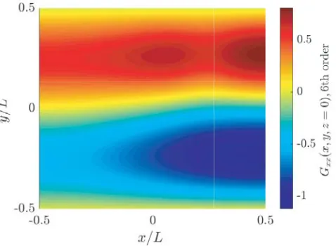
Figure 1 shows the xxcomponent of vector potential dyadic Green’s function over the plane of z = 0 inside the cavity computed by the 6th order convergent summation with imaginary wavenumber extraction. The maximum relative error with respect to the benchmark is less than 10−5 for all of the observation grid points. This result is obtained by including 10 modes (in each direction) in the 6th order summation and 5 clusters of image dipoles to compute the extracted terms with the computational time per observation point of 0.55 msec-CPU.
In order to obtain the same level of accuracy, the Ewald method is also evaluated to reach a relative error of 10−5. The CPU time for this method is 0.76 msec-CPU for evaluation of the dyadic Green’s function at one point.
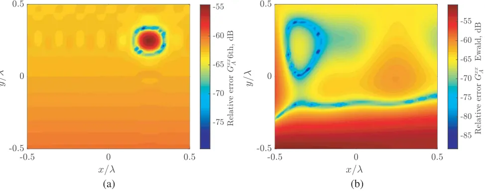
Figure 1. Vector potential Green’s functionGxxA calculated by 6th order convergent spectral expansion, using 6 modes in each direction andξ= 2/L.
(a) (b)
Figure 2. Relative error of 6th order convergent series and Ewald method against the benchmark. (a) 6th order Imaginary extraction. (b) Ewald method.
2.4.2. Second Comparison: Highly Accurate Results
In this part, we set the acceptable error to 10−8 to compare the performance of two approaches. It is clear that the Ewald method performs better if a highly accurate result is desired. The convergence rate of the Ewald method is exponential while the imaginary extraction technique provides 6th order power-law convergence. In order to achieve the desired accuracy, the computation cost of the Ewald and imaginary extraction techniques are 1.7 and 8.2 msec-CPU per point, respectively. Therefore, if a very accurate value of the Green’s function is required, the Ewald sum is superior from the computational cost standpoint.
However, the comparison of the results in Tab. 1 is shown for a single frequency calculation. If a broadband solution of the dyadic Green’s function is required, a very fine frequency sweep should be performed to capture individual resonance lines of the cavity (the resonance lines are closely spaced for a 3-dimensional cavity) that in turn leads to a large number of evaluations of the Green’s function for different frequencies. For example, in order to find the Green’s function of the cavity of dimension
Table 1. Computation cost of 6th order imaginary extraction technique against the Ewald method for different accuracies.
Accuracy Computation cost per point (CPU-msec)
10−5 Ewald 0.76
6th 0.55
10−8 Ewald 1.7
6th 8.2
of resonances. Accounting a few numbers of frequency points to capture a resonance in the Green’s function correctly, the number of required frequency points would be several thousand. However, such a response can be obtained by a single run of the imaginary extraction. For the computational comparison of this wideband example (given required accuracy of 10−5), the expected cost of Ewald method is about 10,000×0.76 CPU·msec while for the imaginary extraction method it only takes 10 CPU·msec including the computation cost for a simple loop over frequency to evaluate the spectral coefficients.
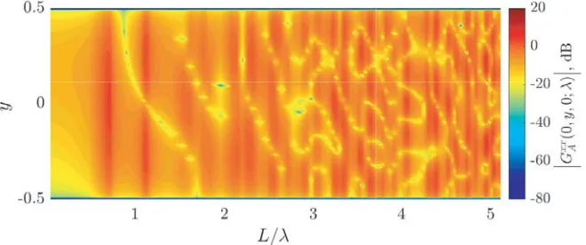
Figure 3 plots the broadband Green’s function for excitation wavelength 0.05≤λ/L≤5 which is 2 decades of bandwidth obtained by imaginary wavenumber extraction technique with only one evaluation of the eigenmodes. The Green’s function is shown over the line x = z = 0 as a function of L/λ for 130 frequency samples. The exact resonant frequencies are avoided as much as possible in plotting the broadband Green’s function for a lossless cavity.
Figure 3. Vector potential Green’s function GxxA(0, y,0;λ) calculated by the 6th order convergent spectral expansion over two decades of bandwidth.
3. ELECTRIC FIELD DYADIC GREEN’S FUNCTION
Given that we have the expression for the vector potential dyadic Green’s function, one may calculate the electric field dyadic Green’s function through Eq. (6). However, it is more insightful to begin with the electric field dyadic Green’s function directly to have a better treatment of its singular behavior in the near field region. The electric field Green’s function G(¯r,¯r) inside the cavity satisfies the vector wave equation of
∇ × ∇ ×G(¯r,r¯)−k20G(¯r,r¯) =Iδ(¯r−¯r) (36)
subject to the Dirichlet boundary condition ˆn×G(¯r ∈ ∂V,r¯) = 0. If we are able to find the vector eigenfunctions ¯Fα(¯r) that satisfy the homogeneous vector wave equation with eigen-wavenumber kα subject to the same type of boundary condition as imposed on the Green’s function, i.e., ˆn×F¯α(¯r ∈
∂V) = 0 such that,
∇ × ∇ ×F¯α(¯r)−k2
then, an eigenmode expansion can be developed for the dyadic Green’s function that satisfies the inhomogeneous vector wave equation. The vector eigenfunctions, which correspond to the Hermitian operator ∇ × ∇ × −k2 (for real values ofk2 and given boundary conditions) constitute a complete and orthogonal basis that spans vector fields in the space that follow the same type of boundary conditions. The idea of completeness can be extended to include generalized functions as well. An eigenfunction expansion of the delta function (which satisfies the corresponding boundary condition on the wave equation operator) can be obtained as
Iδ(¯r−r¯) = α
¯
Fα(¯r) ¯Fα(¯r) (38)
where, it is assumed that the vector eigenfunctions are normalized according to
V d 3¯rF¯
α(¯r)·F¯β∗(¯r) =δαβ (39)
Upon expanding the dyadic Green’s function in terms of vector eigenfunctions and substituting in the inhomogeneous vector wave equation of the dyadic Green’s function we arrive at the similar expansion as the scalar case,
G(¯r,r¯) = α
1
k2 α−k20
¯
Fα(¯r) ¯Fα(¯r) (40)
It is straightforward to verify that the following vector wave functions satisfy the homogeneous vector wave equation as well as the electric field boundary condition on the walls of the cavity.
¯
Mα(¯r) = ∇ ×zψˆ Mα (¯r) ¯
Nα(¯r) = 1
kα∇ × ∇ ×
ˆ
zψN α(¯r)
¯
Lα(¯r) = ∇ψαL(¯r)
where,
ψMα (¯r) =
8
V cos mπ
Lx x+
Lx 2
cosnπ
Ly y+
Ly 2
sinpπ
Lz z+
Lz 2
ψαN(¯r) =
8
V sin mπ
Lx x+
Lx 2
sinnπ
Ly y+
Ly 2
cospπ
Lz z+
Lz 2
ψLα(¯r) =
8
V sin mπ
Lx x+
Lx 2
sinnπ
Ly y+
Ly 2
sinpπ
Lz z+
Lz 2
(41)
The transverse wave functions ¯Mα and ¯Nα are divergence free and with corresponding eigenvalues of
k2
α= mπL x 2 + nπ Ly 2 + pπ Lz 2 (42)
The longitudinal wave functions ¯Lα are curl-free and span the degenerate eigenspace corresponding to the eigenvalue of k = 0. Inclusion of the longitudinal wave functions is critical in the computation of the Green’s function in the source region [28] and beyond that (as will be shown later). If we assume normalized eigenfunctions over the volume of the cavity, the dyadic Green’s function can be written as
G(¯r,r¯) =− 1
k2 0
α ¯
Lα(¯r) ¯Lα(¯r) +
α ¯
Mα(¯r) ¯Mα(¯r) + ¯Nα(¯r) ¯Nα(¯r)
k2 α−k02
(43)
3.1. Normalization of Vector Modes
By taking kx = mπ/Lx, ky = nπ/Ly, kz = pπ/Lz and shifting the center of coordinate system for convenience we have,
¯
Mα·M¯α = ∇ψαM ×zˆ·∇ψαM ×zˆ=−zˆ·∇ψMα ×∇ψαM ×zˆ=|∇ψαM|2− |∇ψMα ·zˆ|2
= 8
V sin2kzz
k2
xsin2kxxcos2kyy+k2ycos2kxxsin2kyy (44)
Therefore,
V d¯r ¯
Mα·M¯α=kαρ2 εmεnεp (45)
whereεn= 1 +δn andkαρ2 = (k2x+ky2). Similarly,
V d¯r ¯
Nα·N¯α =kαρ2 εmεnεp (46)
and for longitudinal wave functions,
V d¯r ¯
Lα·L¯α=kα2εmεnεp. (47)
The dyadic Green’s function in terms of unnormalized vector wave functions ¯M,N¯, and ¯L becomes
G(¯r,r¯) =− 1
k2 0
α 1
εmεnεp 1
k2 α
¯
Lα(¯r) ¯Lα(¯r) +
α 1
εmεnεp 1
k2 αρ
¯
Mα(¯r) ¯Mα(¯r) + ¯Nα(¯r) ¯Nα(¯r)
k2 α−k02
(48)
3.2. Singularity Extraction
In order to extract the singularity of the dyadic Green’s function, let’s consider the asymptotic behavior of each terms asα→ ∞. For ¯Lα term,
lim α→∞
1
k2 α
L¯α(¯r) ¯Lα(¯r) = lim α→∞
1
k2 α
∇(ψα(¯r))∇ψα(¯r)=O(1) (49)
which tends to a constant, but for ¯Mα and ¯Nα terms,
lim α→∞
k12
αρ ¯
Mα(¯r) ¯Mα(¯r)
k2 α−k20
≈ O k12
α lim α→∞ 1 k2 αρ ¯
Nα(¯r) ¯Nα(¯r)
k2 α−k02
≈ O k12
α
(50)
The first term does not represent a convergent series. Since the asymptotic spectral behavior tends to a constant value, it contains a delta function singularity in the spatial domain (which is known as the singularity of the dyadic Green’s function [24–27]). For the free space dyadic Green’s function expansion in terms of continuous spectrum of eigenfunctions, after evaluating one of the spectral integrations by contour integration technique, contribution of the ¯LL¯ term includes a delta function singularity and an static pole term that exactly cancels the static pole hat arise from the ¯NN¯ term [2, 4]. Therefore, the net contribution of the ¯LL¯ term is just a delta function singularity at the source point. However, for the cavity Green’s function where the modes are discrete, the ¯LL¯ term similarly contains a delta function singularity at the source point and a static contribution that extends beyond the source point. The static pole does not appear here for either ¯LL¯ or ¯NN¯ as a consequence of the discrete spectrum. Noting that ψLα =ψα is an eigenfunction of the scalar potential wave equation, and the summation in the ¯LL¯ part of the dyadic Green’s function can be decomposed into two parts: one with all the indices non-zero, and the other contains at least one zero index,
G(¯r,r¯) LL
=−1
k2 0 m,n,p=0 1 k2
α−02∇∇ ψ
α(¯r)ψα(¯r)−k12 0 m,n,p mnp=0 1 k2
α−02∇∇ ψ
α(¯r)ψα(¯r)ε 1
The second term is identically zero. By interchanging the summation and differential operators in the first summation symbolically (the singularity should be taken care of) as
G(¯r,r¯) LL
=−1
k2 0
∇∇
m,n,p=0 1
k2
α−02ψα(¯r)ψα(¯r ) = 1
k2 0
GL(¯r,r¯) (52)
where,
GL(¯r,r¯) =−∇∇Gφ(¯r,r¯;k= 0) (53) that corresponds to the derivative of the scalar Green’s function Gφ(¯r,r¯) of the cavity at DC. Notice thatGL is a frequency-independent part of the dyadic Green’s function G. Using the image expansion of the scalar Green’s function of the cavity
Gφ(¯r,¯r;k= 0) = 1 4π
n,m,p
(−1)n+m+p 1
|r¯−¯rmnp(¯r)| (54)
where ¯rmnp(¯r) is the position of image sources. Taking ¯Rmnp= ¯r−r¯mnp(¯r), then the x-component of the posterior part ofGL for ¯r= ¯r becomes
GL(¯r,r¯)·xˆ= 41π
m,n,p
(−1)n+p 1
R3 mnp
3 ˆRmnpRˆmnp−I
·xˆ (55)
while for they-component of the posterior part, (−1)m+p should be replaced in the summand and so on. This series converges much better than the image expansion of the dynamic dyadic Green’s function. The image expansion of the dynamic dyadic Green’s function is proportional toR−mnp1 while the DC part converges asRmnp−3 versus the number of included images. This term captures the near field singularity of the dyadic Green’s function in the source region. All in all, the dyadic Green’s function for ¯r = ¯r (apart from a delta function singularity at ¯r = ¯r) can be written as
G(¯r,r¯;k0) = 1
k2 0
GL(¯r,r¯) + α
1
k2 αρ
1
εmεnεp ¯
Mα(¯r) ¯Mα(¯r) + ¯Nα(¯r) ¯Nα(¯r)
k2 α−k02
(56)
In addition, a delta function singularity is buried in the definition of GL =−∇∇Gφ(¯r,r¯;k = 0) at ¯r = ¯r. If we consider the image expansion of Eq. (54), singularity comes from the exciting dipole term m =n= p= 0. Therefore, the delta function singularity would be the same as free space case. For ¯r sufficiently close to ¯r, the singular partGLsing can be written as
GLsing(¯r,r¯) =−∇∇ 1 4π|r¯−r¯| =
1 4π∇∇
1
|r¯−¯r| (57)
Applying the trace to both sides of Eq. (57) and noting that Tr∇∇=∇2, it yields TrGLsing=−δ(¯r− ¯
r). Since there is no preference between different directions near the source, Gsing
L =−1/3Iδ(¯r−r¯) and the complete expansion of the dyadic Green’s function that is valid everywhere reads,
G(¯r,¯r;k0) =− 1
3k20Iδ(¯r−r¯ ) + 1
k2 0
GL(¯r,r¯) +
α 1
k2 αρ
1
εmεnεp ¯
Mα(¯r) ¯Mα(¯r) + ¯Nα(¯r) ¯Nα(¯r)
k2 α−k02
(58)
3.3. Spectral Summation Acceleration
Following the imaginary wave number extraction of Eq. (14) and upon subtracting the dyadic Green’s function at the imaginary wave number ofk=iξ from itself yields,
G(¯r,r¯;k) = G(¯r,r¯;iξ) + 1
k2 + 1
ξ2
GL(¯r,r¯)
+
α 1
k2 αρεα
k2+ξ2 (k2
α−k2)(k2α+ξ2) ¯
The DC term does not add any computational effort as it is frequency independent term. In Eq. (59), the imaginary wavenumber extracted termG(¯r,r¯;iξ) will be computed by the image expansion which converges very fast in terms of included images (see Appendix A). The second term GL will be computed by the static image expansion in Eq. (55) which converges much faster than dynamic image expansion. The modal series is now accelerated to the fourth-order of convergence with respect to α. We can proceed to further accelerate the summation by following the same procedure as the vector potential Green’s function,
G(¯r,r¯;k) = G(¯r,r¯;iξ)−k 2+ξ2
2ξ
∂
∂ξG(¯r,r¯;iξ) +
1
k2 + 1
ξ2
GL(¯r,r¯) + k 2+ξ2
2ξ
∂ ∂ξ
−1
ξ2
GL(¯r,r¯)
+
α 1
k2 αρεα
(k2+ξ2)2 (k2
α+ξ2)2(kα2 −k2) ¯
Mα(¯r) ¯Mα(¯r) + ¯Nα(¯r) ¯Nα(¯r) (60)
Again, sinceGL(¯r,r¯) is frequency independent, it leads to a great simplification of the terms,
G(¯r,r¯;k) = G(¯r,¯r;iξ)− k 2+ξ2
2ξ
∂
∂ξG(¯r,r¯;iξ) +
(k2+ξ2)2
k2ξ4 GL(¯r,¯r)
+
α 1
k2 αρεα
(k2+ξ2)2 (k2
α+ξ2)2(kα2 −k2) ¯
Mα(¯r) ¯Mα(¯r) + ¯Nα(¯r) ¯Nα(¯r)
This is the 6th order convergent spectral expansion of the dyadic Green’s function of the rectangular cavity. It only remains to compute the imaginary wavenumber derivative of the dyadic Green’s function. The image expansion of the dyadic Green’s function of the rectangular cavity that is given in the Appendix A can be used to find ∂ξG(¯r,r¯;iξ). Note that for a wideband solution, the extracted terms with imaginary wavenumber as well as the static term GL should be evaluated only one time for a broadband frequency sweep.
Figure 4 plots thexxcomponent of the electric field dyadic Green’s function of the cavity over the plane z= 0 inside the cavity for the exciting wavelength of λ= 0.93L. The source point and physical parameters are the same as the vector potential case in Section 2.4. A wideband evaluation of Gxx is depicted in Fig. 5 with the observation points on the line z = x = 0 in the cavity and the exciting wavelength in the range of 0.05 ≤ λ/L ≤ 5. Notice that the difference between the vector potential
GA and electric field G dyadic Green’s functions is dominant at low frequencies (near field). At high
Figure 5. Electric field dyadic Green’s function Gxx(0, y,0;λ) calculated by 6th order convergent spectral expansion over two decades of bandwidth.
frequencies,
G(¯r,r¯) =
I+∇∇
k2
·GA(¯r,r¯)≈GA(¯r,r¯) (61)
The difference between two dyadic Green’s functions is more pronounced around the source region where the electric field dyadic Green’s function is hyper singular (∝1/R3).
APPENDIX A. IMAGE EXPANSION OF THE DYADIC GREEN’S FUNCTION
The free space Green’s function G0(¯r,r¯;k) at wavenumberk that satisfies the vector wave equation of
∇ × ∇ × −k2G
0(¯r,r¯;k) =Iδ(¯r−r¯) (A1)
subject to the radiation boundary condition at infinity, for ¯r = ¯r can be directly obtained by differentiating the scalar Green’s function as
G0(¯r,r¯;k) = 3
k2R2 − 3i
kR −1
ˆ
RRˆ+ − 1
k2R2 +
i kR + 1
I
G0(R;k) (A2)
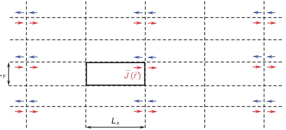
where G0(R;k) = eikR/4πR is the scalar free space Green’s function and R = |r¯−r¯|. In order to obtain the cavity Green’s function that satisfies the Dirichlet boundary condition on the walls, image sources should be placed all around the world in order to produce the response with vanishing tangential component over the walls. Once the boundary conditions are satisfied, presence of the walls does not have any additional effect on the fields, and they can be removed. Fig. A1 shows a 2D profile (xy plane)
Ly
Lx
J (r )'
of the images dipoles around a cross-section of the cavity for ax-directed dipole in the cavity. Changing color from blue to red shows a flip in the sign of the dipole. For ax-directed dipole with unit amplitude, the collective response of all the dipoles in Fig. A1 including the main dipole inside the cavity would be
G⊥(¯r,¯r)·xˆ= mn
(−1)nG0
¯
r;mLx+ (−1)mx, nLy+ (−1)ny, z·xˆ
Here, G⊥(¯r,r¯)·xˆ is the collective response of the image dipoles for a plane perpendicular to z; the source dipole is located at (x, y, z) inside the cavity; (mLx + (−1)mx, nLy + (−1)ny, z) is the location of the image dipoles for 2D profile of Fig. A1; andG0 is the free space dyadic Green’s function. Taking the other two walls into account yields,
G(¯r,r¯)·xˆ = p
(−1)pG⊥(¯r,r¯p)·xˆ
=
m,n,p
(−1)n+pG0
¯
r;mLx+ (−1)mx, nLy+ (−1)ny, pLz+ (−1)pz
·xˆ (A3)
For real values of k, Eq. (A3) has a slow convergence rate that makes it not an attractive way of computing the cavity Green’s function. However, for an imaginary wavenumber k = iξ, it has an exponential convergence rate. In this case, the free space dyadic Green’s function becomes
G0(¯r,r¯;iξ) =
− Q32 + 3
Q + 1
ˆ
RRˆ+ 1
Q2 + 1
Q+ 1
I
ξe−Q
4πQ (A4)
where Q = ξR and R is the distance between the source and observation points. Similarly, for the wavenumber derivative of the dyadic Green’s function, the image expansion of Eq. (A3) can be evaluated with considering
∂
∂ξG0(¯r,r¯;iξ) = e −Q
4π
6
Q3 + 6
Q2 + 3
Q+ 1
ˆ
RRˆ− 2
Q3 + 2
Q2 + 1
Q+ 1
I
(A5)
that is still exponentially convergent.
REFERENCES
1. Tai, C.-T., “Dyadic Green functions in electromagnetic theory,”Institute of Electrical&Electronics
Engineers, IEEE, 1994.
2. Collin, R. E.,Field Theory of Guided Waves, McGraw-Hill, New York, 1960.
3. Felsen, L. B. and N. Marcuvitz, Radiation and Scattering of Waves, Vol. 31, John Wiley & Sons, 1994.
4. Chew, W. C.,Waves and Fields in Inhomogeneous Media, IEEE Press, 1995.
5. Marliani, F. and A. Ciccolella, “Computationally efficient expressions of the dyadic Green’s function for rectangular enclosures,” Progress In Electromagnetics Research, Vol. 31, 195–223, 2001. 6. Park, M.-J. and S. Nam, “Rapid summation of the Green’s function for the rectangular waveguide,”
IEEE Transactions on Microwave Theory and Techniques, Vol. 46, No. 12, 2164–2166, 1998.
7. Araneo, R. and G. Lovat, “An efficient mom formulation for the evaluation of the shielding effectiveness of rectangular enclosures with thin and thick apertures,” IEEE Transactions on
Electromagnetic Compatibility, Vol. 50, No. 2, 294–304, 2008.
8. Hill, D. A., Electromagnetic Fields in Cavities: Deterministic and Statistical Theories, Vol. 35, John Wiley & Sons, 2009.
9. Soler, F. J. P., F. D. Q. Pereira, D. Ca nete Rebenaque, Alejandro Alvarez Melcon, and Juan R Mosig, “A novel efficient technique for the calculation of the Green’s functions in rectangular waveguides based on accelerated series decomposition,” IEEE Transactions on Antennas and
Propagation, Vol. 56, No. 10, 3260–3270, 2008.
10. Park, M.-J., “Accelerated summation of the Green’s function for the rectangular cavity,” IEEE
11. Gruber, M. E. and T. F. Eibert, “A hybrid ewald-spectral cavity Green’s function boundary element method with spectral domain acceleration for modeling of over-moded cavities,”IEEE Transactions
on Antennas and Propagation, Vol. 63, No. 6, 2627–2635, 2015.
12. Campione, S. and F. Capolino, “Ewald method for 3D periodic dyadic Green’s functions and complex modes in composite materials made of spherical particles under the dual dipole approximation,” Radio Science, Vol. 47, No. 6, 1–11, 2012.
13. Borji, A. and S. Safavi-Naeini, “Rapid calculation of the Green’s function in a rectangular enclosure with application to conductor loaded cavity resonators,” IEEE Transactions on Microwave Theory
and Techniques, Vol. 52, No. 7, 1724–1731, 2004.
14. Tsang, L. and S. Huang, “Broadband Green’s function with low wavenumber extraction for arbitrary shaped waveguide and applications to modeling of vias in finite power/ground plane,”
Progress In Electromagnetics Research, Vol. 152, 105–125, 2015.
15. Tan, S. and L. Tsang, “Green’s functions, including scatterers, for photonic crystals and metamaterials,” JOSA B, Vol. 34, No. 7, 1450–1458, 2017.
16. Tan, S. and L. Tsang, “Scattering of waves by a half-space of periodic scatterers using broadband green’s function,”Optics Letters, Vol. 42, No. 22, 4667–4670, 2017.
17. Tan, S. and L. Tsang, “Efficient broadband evaluations of lattice Green’s functions via imaginary wavenumber components extractions,” Progress In Electromagnetics Research, Vol. 164, 63–74, 2019.
18. Tsang, L. and S. Tan, “Calculations of band diagrams and low frequency dispersion relations of 2D periodic dielectric scatterers using broadband Green’s function with low wavenumber extraction (BBG),” Optics Express, Vol. 24, No. 2, 945–965, 2016.
19. Huang, S. and L. Tsang, “Fast electromagnetic analysis of emissions from printed circuit board using broadband Green’s function method,”IEEE Transactions on Electromagnetic Compatibility, Vol. 58, No. 5, 1642–1652, 2016.
20. Arcioni, P., M. Bozzi, M. Bressan, G. Conciauro, and L. Perregrini, “The BI-RME method: An historical overview,” 2014 International Conference on Numerical Electromagnetic Modeling and
Optimization for RF, Microwave, and Terahertz Applications (NEMO), 1–4, IEEE, 2014.
21. Bozzi, M., L. Perregrini, and K. Wu, “Modeling of conductor, dielectric, and radiation losses in substrate integrated waveguide by the boundary integral-resonant mode expansion method,”IEEE
Transactions on Microwave Theory and Techniques, Vol. 56, No. 12, 3153–3161, 2008.
22. Guglielmi, M., R. Sorrentino, and G. Conciauro, Advanced Modal Analysis: CAD Techniques for
Waveguide Components and Filter, John Wiley & Sons, Inc., 1999.
23. Tsang, L., K.-H. Ding, T.-H. Liao, and S. Huang, “Modeling of scattering in arbitrary-shape waveguide using broadband Green’s function with higher order low wavenumber extractions,”IEEE
Transactions on Electromagnetic Compatibility, Vol. 60, No. 1, 16–25, 2017.
24. Chew, W. C., “Some observations on the spatial and eigenfunction representations of dyadic Green’s functions (electromagnetic theory),” IEEE Transactions on Antennas and Propagation, Vol. 37, No. 10, 1322–1327, 1989.
25. Wang, J., “A unified and consistent view on the singularities of the electric dyadic Green’s function in the source region,” IEEE Transactions on Antennas and Propagation, Vol. 30, No. 3, 463–468, 1982.
26. Yaghjian, A. D., “Electric dyadic Green’s functions in the source region,”Proceedings of the IEEE, Vol. 68, No. 2, 248–263, 1980.
27. Johnson, W. A., A. Q. Howard, and D. G. Dudley, “On the irrotational component of the electric Green’s dyadic,” Radio Science, Vol. 14, No. 6, 961–967, 1979.