Detection and Localization of an Object behind Wall Using an
Inverse Scattering Technique with Wall Direct Subtraction Method
Mohamad Faizal Mahsen, Kismet Anak Hong Ping*, and Shafrida Sahrani
Abstract—Through-wall imaging (TWI) is one of the useful applications nowadays in microwave tomography field. Reconstructing image of an object becomes more challenging when it is obscured by walls. In practice, the inclusions of noise worsen the reconstruction results. In this paper, Forward-Backward Time-Stepping (FBTS) in time inversion technique is utilized and integrated with Wall Direct Subtraction (WDS) method to reconstruct unknown object behind walls. The investigation includes two types of walls that are homogeneous and heterogeneous. The object is surrounded by closed walls. With noise added in the setup, Singular Value Decomposition (SVD) and Savitzky-Golay (SG) filtering method are used to eliminate the noise and enhance the reconstructed image of an object. The results show that WDS integrated with FBTS has successfully mitigating wall clutter from both homogeneous and heterogeneous walls, and also improves image reconstruction of a hidden object. Further, by using the proposed noise reduction method, lower MSE values can be achieved.
1. INTRODUCTION
A classic ground-penetrating radar application aims to detect buried landmines by probing the ground at multiple locations. It faces a challenge due to the reflection of a large number of incident waves from the surface of the ground [1]. Microwave is widely used in the infrastructure industry, military [2], and bio-medical fields [3]. It is considered that part of the electromagnetic spectrum between 300 MHz and 300 GHz, and most microwave engineering take place from 1 to 40 GHz [4]. It is employed in a host of applications including homeland security, determination of building layout from outdoors (e.g., TWI), civil structure monitoring [5] and breast cancer detection [6, 7].
To obtain images with better resolution and information, setup parameters such as large arrays of antenna and appropriate excitation frequency are required [8]. As a result, extended time duration is needed which may change the positions, smearing and blurring the reconstructed image. For frequency ranging from a few hundred megahertz to 2–3 GHz, most of the building materials are relatively transparent, and this makes high-resolution TWI feasible [9]. Generally, the excitation source for microwave systems utilizes either continuous wave, stepped frequency continuous wave (SFCW), or pulse wave [10].
There are many reconstruction techniques utilizing RADAR, X-Ray, Doppler, and microwaves to detect hidden object behind wall. There are also a number of TWI techniques that have been developed for example in [11–16]. Most of these techniques assume the exact knowledge or estimated wall parameters. In most TWI applications, the wall characteristics are unknown, and the wall is an inhomogeneous and periodic-like structure [17, 18]. TWI structures can be identified by the analysis software based on different techniques such as short electromagnetic pulses, holographic, real aperture, projection and diffraction tomographic reconstruction, and near-field methods [19].
Received 7 January 2019, Accepted 14 May 2019, Scheduled 5 August 2019
* Corresponding author: Kismet Anak Hong Ping ([email protected]).
Wall clutter distorts the return signal from the object resulting in masking of the image of object, particularly when the object is in close proximity to the wall [20]. Imaging process must be able to reconstruct images of object without any distortions and inaccuracy due to the presence of the wall. Several linear inversion scheme based methods for image reconstructions are physical optic approximation [21], back projection [22], and Born approximation [11, 23].
Some research works in TWI focus on different aspects such as wall parameter estimation [24], effect of wall structure [17], obscured object refinement (shape, size, electrical properties and location) [25], and time of processing.
The reconstructed image of obscure target, for example, using wavelet transforms (WT) and singular value decomposition (SVD) based clutter reduction method has been presented in [26]. SVD is used to reduce wall clutter while WT is employed to further suppress the noise. The reconstructed image from a linear combination of the wavelet functions and its coefficients successfully detects multiple objects in heavy clutter environment.
A spatial filtering method as reported in [1] has been applied across the antenna array to mitigate wall reflections. It is tested with solid wall, multilayered wall, and cinder block wall. Spatial filtering is dependent on horizontal-vertical invariance of wall characteristics. It specifically works with infinite impulse response (IIR) notch filter across the array aperture, which removes zero-frequency content. The filtering technique operated in low frequencies is only limited for homogeneous or near-homogeneous wall type [27].
In [28], the time-reversal (TR) method is used to detect and localize object behind wall that shows an improved result based on Target Initial Reflection method. This method is the enhancement of Maximum E-field method [29] and Entropy-based method [30] which provides maximum amplitude of obscured object for detection and localization. Specifically, it solves the issue of finding an optimum period where the object can be configured in TWI system. The utilization of minimum entropy criterion in TWI algorithm has also been presented in [31, 32]. The image degradation occurs if the focusing time is unsuitably selected, which causes leading or lagging of optimal focusing time [33].
EM parameters of the wall such as insertion loss, dielectric constant, loss tangent, reflection and transmission coefficients are very useful in representing wall characteristics. Muqaibel et al. [34] have reported that insertion transfer function can compensate wall clutter. Their work estimates wall characteristic that is free from the effect of wall clutter on object localization.
The time domain technique has the ability to reconstruct an accurate profile of electrical properties as in the FBTS technique, compared to frequency domain based technique. Thus, the FBTS technique has been used for the detection of breast cancer [6, 7, 35], tumors in the lung [36], and tumors in the brain [37]. Following the advancement of FBTS, filters such as Elliptic filter [38] and Chebyshev filter [39] are incorporated to solve the non-linearity problem. In addition, regularization techniques are also integrated into FBTS as described in [40, 41] to handle the quantitative information with an ill-posed or ill-conditioning problem. Regularization techniques are able to provide higher accuracy of electrical properties profile, object shapes, and location. Other promising techniques introduced in [42] propose the inversion method that efficiently handles the strong non-linearity of inverse scattering problem in the inhomogeneous medium using difference Lippmann-Schwinger integral equation (D-LSIE) and difference new integral equation (D-NIE).
In a practical situation, noise is one of the factors other than wall clutter that can distort the reconstructed image of an object. Enhancement of signal to noise ratio (SNR) can be carried out by either hardware or software techniques. The common method in reducing noise is by using a filter. Chebyshev Low Pass Filter (CLPF) as in [39] suppresses the noise located at higher frequency region, reducing the noise effect and improving the reconstructed image of an object. To apply CLPF, time domain signal is transformed into frequency domain before high frequency of noise is removed. As reported in [43], SVD and SG filters are other alternatives to enhance signals. It is shown that the noise in time-domain is successfully reduced, which is better than Low Pass Filter and Wiener Filter.
based filter. This paper is organized as follows. Section 2 describes the setup of the simulation including the geometry and specifications of the space domain, WDS method to mitigate wall clutter, and noise reduction techniques based on SVD and SG filtering. In Section 3, we address analysis of the proposed method for different domain setups, wall types, and noise reduction performances with different wall parameters and noise levels. Lastly, Section 4 concludes the work and provides suggestion for future improvement.
2. SIMULATION SETUP
The research focuses on the development of a microwave TWI system synthetically utilizing FBTS [6] to reconstruct images and detect hidden object.
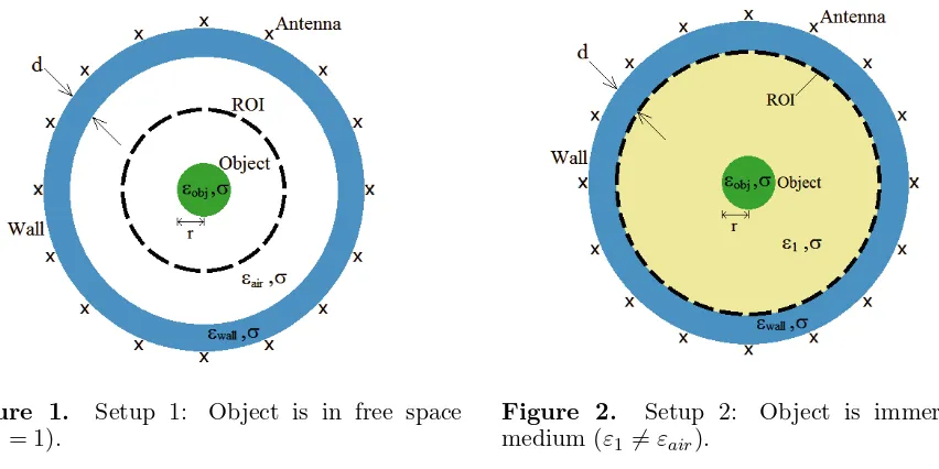
Figure 1. Setup 1: Object is in free space (εair= 1).
Figure 2. Setup 2: Object is immersed in medium (ε1 =εair).
The simulation work operates in transverse magnetic (TM) inverse scattering assuming no induced magnetic source. The TWI simulation setups in 2D are shown in Figure 1 and Figure 2, respectively. The geometry of the setup comprises a circular closed wall with thickness, dcm, and a circular object is located at the center of the domain, with radiusr of 5 cm. Region-of-Interest (ROI) is set tol1cm in radius. The relative permittivities for wall and object are denoted asεr(wall) andεr(object), respectively. The size of the computational domain is 160×160 cm2; cell size is 1×1 cm2; and the thickness of Convolutional Perfectly Matched Layer (CPML) as an Absorber Boundary Condition (ABC) is set to 15 cm on each side. There are 16 point source antennas positioned a centimeter away from the outer wall surface. Each point source antenna is positioned equidistantly atrtm(m = 1,2, . . . , M) in circular form. Only one transmitter transmits a signal at a time while other remaining antennas positioned at
rnr(n= 1,2, . . . , N) act as receivers. The total combination of transmitter/receiver data set is M ×N
(16×15 = 240). Sinusoidal modulated Gaussian pulse is used as an excitation source with bandwidth,
B, of 1.3 GHz and center frequency, fc, of 1 GHz. Another setup as illustrated in Figure 2 comprises a
dcm thickness of circular closed wall, a circular object with radiusr= 5 cm located at the centre of the domain, and a medium in between with electrical permittivity, ε1. The radius of ROI in this setup is set tol2cm. The wall condition in Setup 2 has been investigated further with heterogeneous type. The total signal at each receiver can be expressed as,
um(o)(p;rrn, t) = kmn(t)
vm(fs)(p;rrn, t)−v˜m(rrn, t)
(1)
that takes a value of zero att=ttotal. In this research work, all simulations are carried out by utilizing a single computing; algorithm is written in C++ language; and MATLAB software is used to represent the reconstructed image for evaluation and analysis purposes.
2.1. Wall Direct Subtraction
The measured signals as expressed in Equation (1) have been contaminated with wall clutter. To remove the wall clutter, WDS method is employed. Detail of this method can be found in [44]. In this work, the electrical properties and thickness of the homogeneous wall are considered a priori known. Two TWI setups as illustrated in Figure 1 and Figure 2 have been used in order to investigate the performance of WDS. The calculated electromagnetic fields with the inclusion of known wall parameter inpis expressed as,
vm(w)(p;rrn, t) (3)
The scattered fields from an object can be achieved by subtracting Equation (3) from Equation (1) instead of calculated electromagnetic field in free space. The weighted scattered fields from an object are given by,
um(o)(p;rrn, t) =kmn(t)
vm(w)(p;rrn, t)−v˜m(rrn, t)
(4)
2.2. Noise Reduction
In this work, the noise is added at the receivers to form contaminated signals. For this condition, the received signals are included with uniformly distributed random noise as in Equation (5). Common spectrum of noise is expected to inhabit at high frequency. Based on Equation (4), it can further be expressed when the noise is contaminating the total received signals,
um(o+noise)(p;rrn, t) =um(o)(p;rrn, t) +kmn(t){Hm(rrn, t)} (5) whereHm(rrn, t) is the additive white noise function.
To eliminate the noise, SVD based method is used to exclude the noise subspace. After the noise reduction process, the FBTS is used to reconstruct the image of the object in ROI. The details of this method can be found in [6]. Equation (6) shows the signal-to-noise ratio (SNR) between measured electromagnetic fields and the additive noise. T is a time duration of the measurement.
SNR = 10log10 M m=1 N n=1 T 0
v˜m(rtn, t)2dt
M m=1 N n=1 T 0
Hm(rtn, t)2dt
(6)
2.2.1. Singular Value Decomposition
There are 16 antennas as point source used in this numerical work, which provide 240 data sets. Before SVD is applied, the scattered fields as data matrix is constructed by using Equation (7).
D= [d11 d21 d31 . . . dnm] (7) wherednm is scattered fields data from the nth receiver by themth transmitter. The dimension of this scattered fields data matrix, D, is m×n where m ≥ n. Some useful properties of SVD are applied to any type of matrices and optimality property. In this research, all scattered signals are arranged in a matrix as in Equation (7). SVD application on scattered data matrix D with dimensionm×nis,
D=U·S·VT (8)
2.2.2. Singular Value Elimination
In [43], noise can be eliminated by means of enhancement of an input scattering data matrix using SVD. The diagonal singular value matrixSwill be used to eliminate the noise subspace. From [45], it is shown that the signal from a point target spans several eigen-components, and the number of non-zero singular values depends on the location of the target. The obscured object and noise signal span in different subspaces as
S=
SSc 0 0 Snoise
(9)
whereSSc is the object scattered subspace, andSnoise is the noise subspace.
Through observation, when there is no noise added, the first few sets of eigen-components will have higher singular values. Eigen-components will span when the noise is added. The singular values decomposed from SVD will have a non-increasing arrangement,si = (s1, s2, s3, s4, . . . , sk), wherekis the matrix rank. Based on [43], the noise subspace is usually located at higher index. The threshold point is a boundary between SSc andSnoise which can be identified from the singular values curve. The empirical threshold index will be used to determine the number of singular values to be retained, as in Equation (10).
sk = si ifk≤threshold index
0 elsewhere (10)
The new set of singular values, sk, provides a new set of singular value matrix S with rank, k. MatrixS is used to compose the new enhanced input matrix. The subspace is filtered by using Singular Value Elimination (SVE) technique that has been proven effective in the area of signal enhancement [43]. In Equation (11), matricesS,U, andVT contain the first subspace of the scattered fields while the rest will be the noise subspace.
D=U·S·VT=
USc Unoise ·
SSc 0
0 Snoise
·
VScT VTnoise
(11)
By eliminating noise subspace in singular value matrix based on Equation (10), the enhanced scattered data matrix using SVE,DSVE can be expressed as,
DSVE =
USc Unoise
·
SSc 0
0 0 · VT Sc VTnoise
=U·S·VT (12)
As discussed in [43], elimination process of some singular values still contains residual noise in the signal subspace. Thus, distortion of the reconstructed image, caused by the residual noise, needs to be minimized. Savitzky-Golay Filter is used to handle the filtering process.
2.2.3. Savitzky-Golay Filter
Noise reduction is necessary to eliminate residual noise that exists in both left,Uand right,V singular vector matrices. This method has been discussed in [46, 47] and applied in [48, 49]. Savitzky-Golay (SG) filter has been chosen due to its capability to work in time-series and preserve the features. This filtering method is an improved version of moving average (MA) technique, by updating the data based on polynomial fitting. The range of data to be updated is known as window denoted asw. The degree or order of polynomial used in the fitting is denoted as n. Thus, SG filter is applied at Ui and Vi, column by column as
SG{Ui}=Ui (13)
SG{Vi}=Vi (14)
whereiis the number of columns.
Ui and Vi are the filtered data matrices for left and right singular vectors. The next step is to rebuild the enhanced scattered data matrix as,
3. NUMERICAL ANALYSIS
3.1. Wall Direct Subtraction
The reconstruction of hidden object can be performed utilizing FBTS with WDS method. Numerical work includes the effect of different wall characteristics such as thickness, type of wall, and electrical properties.
3.1.1. Homogeneous Wall
The known wall parameter is considered homogeneous with uniform thickness. The numerical results presented in Figure 3 show relative permittivity profiles of hidden object behind the two types of wall, homogeneous and heterogeneous wall.
(a) (b)
(c) (d)
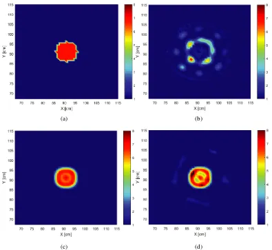
Figure 3. Reconstructed image with Setup 1. (a) Actual hidden object behind wall. (b) Poorly reconstructed image without WDS. (c) Reconstructed image behind homogenous wall with WDS. (d) Reconstructed image behind heterogeneous wall with WDS.
Figure 3(b) shows the result of a poorly reconstructed image when no WDS is applied, while Figure 3(c) and Figure 3(d) show an improved image reconstruction of a hidden object when FBTS is incorporated with WDS. Reconstructed image profile behind heterogeneous wall is found more uneven than that behind homogenous wall. Mean Square Error (MSE) values for the results in Figure 3(b), Figure 3(c), and Figure 3(d) are 1.6007, 0.0066, and 0.0150, respectively. The numerical simulation, as in Figure 3, is considered free from noise. Similar numerical tests have been applied with Gaussian Noise and discussed in Subsection 3.2.
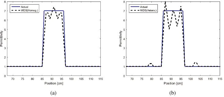
Figure 4 shows the cross-sectional views of reconstruction of hidden object behind homogenous and heterogeneous walls. Results prove that if the wall parameter used in WDS is accurately selected, the reconstruction will be in its maximum performance with minimum distortion. Subsection 3.1.2 presents two types of walls with the object immersed in a medium.
(a) (b)
Figure 4. Cross-sectional view atx= 90 of reconstructed image using WDS. (a) Reconstructed image behind homogenous wall. (b) Reconstructed image behind heterogeneous wall.
3.1.2. Wall with Hidden Object Immersed in a Medium
For further investigation, the object is immersed in a medium (εr = 1) as illustrated in Figure 2. The transmitted wave propagating via layered and different media increases the degradation of signals at receiver. Two respective simulations have been carried out with different walls. An object is immersed in a medium with relative permittivity εr of 10 and conductivity σ of 0.001 S/m. For Setup 2, the simulation involves the heterogeneous wall as listed in Table 1.
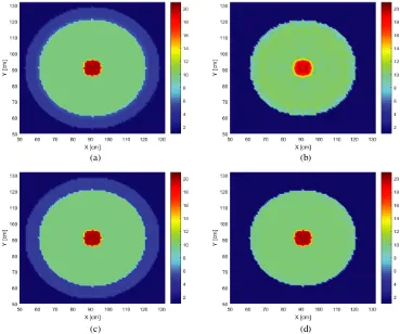
Figure 5 shows reconstructed images with Setup 2 for both Wall Type 1 and Type 2. Figure 6 shows the cross-sectional views of reconstructed image of object for Wall Type 1 and Wall Type 2.
Table 1. Heterogeneous wall type.
Wall Type Description
1. Two-Layer
Outer layer: Thickness,d1 of 6 cm Permittivity,εr1 of 5
Inner layer: Thickness,d2 of 2 cm Permittivity,εr2 of 5.5
(c) (d) (a) (b)
Figure 5. Reconstructed image with Setup 2. (a) Actual object behind Wall Type 1. (b) Reconstructed image behind Wall Type 1. (c) Actual object behind Wall Type 2. (d) Reconstructed image behind Wall Type 2.
(a) (b)
Figure 6. Cross-sectional view of atx= 90 of Setup 2 with (a) Wall Type 1 and (b) Wall Type 2.
Although the reconstruction of an object is barely viable, the electrical properties of the reconstructed image are acceptable.
3.2. Noise Reduction
The performance of SVE with SG (SVE-SG) technique in reducing noise of image reconstruction can be expressed quantitatively using MSE.
MSE =1 Q
Q
i=1
{Gi−Hi}2 (16)
whereQis the total number of cells or data in the ROI region. The details of actual and reconstructed image at theith cell are denoted asHi and Gi, respectively.
SVE-SG method is a combination of two processes in eliminating noise, namely SVE and SG. By eliminating the higher singular values using SVE and retain the rest as described in Equation (10), reduction of noise subspace can be achieved. The threshold index with the approximate value of less than 10 is chosen in order to eliminate the higher index in this research work. This procedure is set based on observation as described in [43]. To further reduce the noise, Left and Right Singular Vectors are filtered by using SG with suitablew andn values.
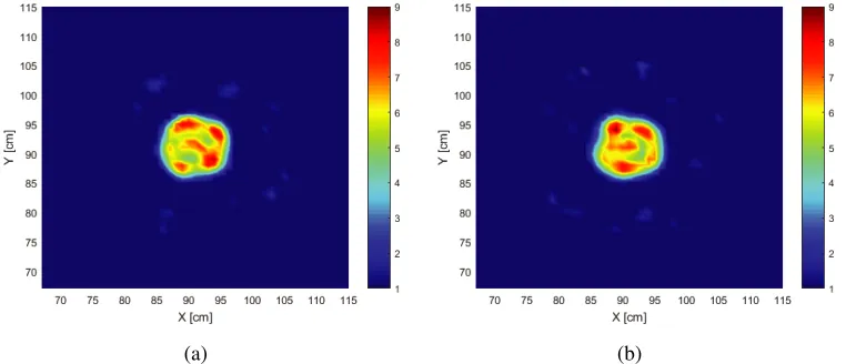
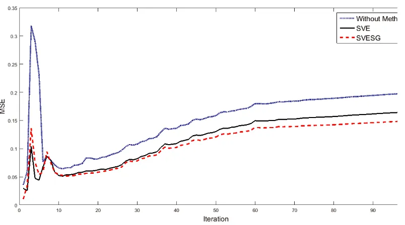
A few noise levels are applied to demonstrate the performance of noise reduction using SVE-SG. As an example, Figure 7 shows the reconstructed image of an object when−3 dB Gaussian noise is added before and after the SVE-SG method is applied. To validate the performance of the noise reduction method with SVE-SG, MSE is used as in Equation (16). It shows that SVE-SG effectively reduces the noise with SNR of −3 dB, 3 dB, 6 dB, and 10 dB by 24.90%, 19.43%, 3.25%, and 42.23%, respectively. Figure 8 shows the MSE curve for noise with SNR of −3 dB without SVE-SG, with SVE and with SVE-SG.
(a) (b)
Figure 7. Reconstruction of object by FBTS-WDS in noise with SNR =−3 dB. (a) Without SVE-SG (MSE = 0.1992). (b) With SVE-SG (MSE = 0.1496).
As shown in Figure 8, MSE curve for SVE-SG is lower than the MSE curve without SVE-SG. This concludes that the SVE-SG successfully eliminates the noise. For these results, SVE-SG depends on the threshold index, wand n of the polynomial.
3.3. MSE Analysis
Figure 8. MSE value at each iteration in noise with SNR of−3 dB.
3.3.1. Wall Thickness
The signals propagating through walls will be distorted and degraded further depending on wall thickness. The increment of signal attenuation is proportional to wall thickness of the same material. In Setup 1 as noise is added, the performances of SVE and SVE-SG are recorded with different wall thicknesses as shown in Table 2. The MSE values have been calculated for without noise reduction (Without Method), with SVE and SVE-SG methods, respectively.
Table 2. MSE for different wall thickness.
Wall Thickness(cm) Without Method SVE SVE-SG
2 0.5261 0.2796 0.1909
5 0.4734 0.1324 0.0805
10 0.1992 0.1659 0.1496
Table 3. MSE with different wall permittivity.
Wall Permittivity, εr(wall) Without Method SVE SVE-SG
4 0.3677 0.3170 0.2844
6 0.4314 0.3308 0.1047
8 0.1289 0.0871 0.0631
10 0.1624 0.0633 0.0508
3.3.2. Wall Electrical Properties
Degradation of signals also occurs when permittivity of the wall is changed. Table 3 shows the result of the investigation on the effect of different wall permittivity values (4 to 10), with respective MSE. As an example with permittivity εr(wall) of 8, it provides 32.43% reduction of noise with SVE method only. When SVE-SG is applied, noise reduction improves with noise reduction increased to 51.05%.
4. CONCLUSION
This research has focused on the reconstruction of a hidden object using FBTS for TWI application. Several investigations have been carried out including object immersed in a different medium and different wall parameters (thickness and electrical properties). A simple circular wall structure is assumed in this research work, where the complexity of wall structure (e.g., single-sided, corners or cinder-block walls) can be avoided and at the same time to focus on the performance of the proposed method. The future steps of research work will comprise a more challenging wall structure.
The ability of FBTS with WDS in this paper will stand as a platform for any TWI or Non-Destructive Testing (NDT) application utilizing FBTS, to optimize the accuracy of image reconstruction profile. A priori known wall parameter used in FBTS with WDS can be further improved using an enhanced estimation method. This method integrated with FBTS is capable of solving a problem to mitigate wall clutter of unknown parameters.
SVD based filter successfully reduces noise in the scattered field, with enhanced reconstruction profile. The SVD filtering method can be used on any time-domain data sets, and it can preserve the shapes of the signals.
ACKNOWLEDGMENT
The authors would like to thank UNIMAS for the valuable support throughout the research work.
REFERENCES
1. Yoon, Y. and M. G. Amin, “Spatial filtering for wall-clutter mitigation in through-the-wall radar imaging,”IEEE Trans. Geosci. Remote Sens., Vol. 47, No. 9, 3192–3208, 2009.
2. Baranoski, E. J. and N. F. Drive, “Through wall imaging: Historical perspective and future directions,”J. Franklin Inst., Vol. 345, No. 6, 556–569, 2008.
3. Salvador, S. M., E. C. Fear, M. Okoniewski, and J. R. Matyas, “Exploring joint tissues with microwave imaging,” IEEE Trans. Microw. Theory Tech., Vol. 58, No. 8, 2307–2313, 2010.
4. Wentworth, S. M., Fundamentals of Electromagnetics with Engineering Applications, John Wiley & Sons, Inc., USA, 2005.
5. Syahrim, N. and N. Anwar, “Multiple line cracks in concrete material,” Int. J. Hum. Technol. Interact., Vol. 2, October 2018.
6. Hong Ping, K. A., T. Moriyama, T. Takenaka, and T. Tanaka, “Reconstruction of breast composition in a free space utilizing 2-D forward-backward time-stepping for breast cancer detection,” Adv. Medical, Signal Inf. Process. 2008 (MEDSIP 2008), 4th lET Intematioal Conf., 1–4, 2008.
7. Hong, K. A., T. Moriyama, T. Takenaka, and T. Tanaka, “Two-dimensional forward-backward time-stepping approach for tumor detection in dispersive breast tissues,” Microw. Symp. (MMS), 2009 Mediterr., 2009.
8. Kaushal, S. and D. Singh, “Sensitivity analysis of microwave UWB radar for TWI system,”Int. J. Appl. Eng. Res., Vol. 12, No. 19, 8665–8675, 2017.
10. Gaikwad, A. N., D. Singh, and M. J. Nigam, “Application of clutter reduction techniques for detection of metallic and low dielectric target behind the brick wall by stepped frequency continuous wave radar in ultra-wideband range,” IET Radar, Sonar Navig., Vol. 5, 416–425, 2011.
11. Soldovieri, F. and R. Solimene, “Through-wall imaging via a linear inverse scattering algorithm,”
IEEE Geosci. Remote Sens. Lett., Vol. 4, No. 4, 513–517, 2007.
12. Dehmollaian, M. and K. Sarabandi, “Refocusing through building walls using synthetic aperture radar,”IEEE Trans. Geosci. Remote Sens., Vol. 46, No. 6, 1589–1599, 2008.
13. Ahmad, F., S. Member, M. G. Amin, and G. Mandapati, “Autofocusing of through-the-wall radar imagery under unknown wall characteristics,” IEEE Trans. Signal Process., Vol. 16, No. 7, 1785– 1795, 2007.
14. Paknys, R., “Reflection and transmission by reinforced concrete — Numerical and asymptotic analysis,”IEEE Trans. Antennas Propag., Vol. 51, No. 10, 2852–2861, 2003.
15. Liang, F., et al., “Through the wall imaging of human vital signs based on UWB MIMO bioradar,”
Progress In Electromagnetics Research C, Vol. 87, 119–133, 2018.
16. Jia, S., L. Kong, and Y. Jia, “A new approach for target localization of through-the-wall radar with unknown walls,” IEEE Natl. Radar Conf. — Proc., No. 3, 7–10, 2009.
17. Gennarelli, G. and F. Soldovieri, “Radar imaging through cinderblock walls: Achievable performance by a model-corrected linear inverse scattering approach,”IEEE Trans. Geosci. Remote Sens., Vol. 52, No. 10, 6738–6749, 2014.
18. Burkholder, R. J., R. J. Marhefka, and J. L. Volakis, “Radar imaging through cinder block walls and other periodic structures,” 2008 IEEE Antennas Propag. Soc. Int. Symp., 3–6, 2008.
19. Turk, A. S., K. A. Hocaoglu, and A. A. Vertiy,Subsurface Sensing, Volume 197 of Wiley Series in Microwave and Optical Engineering, John Wiley & Sons, 2011.
20. Yemelyanov, K. M., N. Engheta, A. Hoorfar, and J. A. Mcvay, “Adaptive polarization contrast techniques for through-wall microwave imaging applications,”IEEE Trans. Geosci. Remote Sens., Vol. 47, No. 5, 1362–1374, 2009.
21. Pierri, R., A. Liseno, R. Solimene, and F. Soldovieri, “Beyond physical optics SVD shape reconstruction of metallic cylinders,” IEEE Trans. Antennas Propag., Vol. 54, No. 2, 655–665, 2006.
22. Zhong, W. and C. Tong, “A novel near field imaging approach for through-wall imaging,” Cross Strait Quad-Regional Radio Sci. Wirel. Technol. Conf., 164–167, 2011.
23. Miao, Z. and P. Kosmas, “Cmpact of information loss on reconstruction quality in microwave tomography for medical imaging,” Diagnostics, Vol. 8, No. 52, 1–15, 2018.
24. Jin, T., B. Chen, and Z. Zhou, “Image-domain estimation of wall parameters for autofocusing of through-the-wall SAR imagery,” IEEE Trans. Geosci. Remote Sens., Vol. 51, No. 3, 1836–1843, 2013.
25. Liseno, A., F. Soldovieri, and R. Pierri, “Improving a shape reconstruction algorithm with thresholds and multi-view data,” AEU — Int. J. Electron. Commun., Vol. 58, No. 2, 118–124, 2004.
26. Riaz, M. M. and A. Ghafoor, “Wavelet transform and singular value decomposition based clutter reduction for through wall imaging,”Radar Conf. IET Int., 2013.
27. Tivive, F. H. C., M. G. Amin, and A. Bouzerdoum, “Wall clutter mitigation based on eigen-analysis in through-the-wall radar imaging,” 17th DSP 2011 Int. Conf. Digit. Signal Process. Proc., 1–8, 2011.
28. Gorji, A. B. and B. Zakeri, “An improved time-reversal-based target localization for through-wall microwave imaging,”J. Electr. Comput. Eng. Innov. JECEI Regul. Pap. 89 J. Elec. Comput. Eng. Innov., Vol. 1, No. 2, 89–97, 2013.
30. Cresp, A., I. Aliferis, M. Yedlin, C. Pichot, and J. Dauvignac, “Investigation of time-reversal processing for surface-penetrating radar detection in a multiple-target configuration,” Proc. 5th Eur. Radar Conf. Amsterdam, Netherlands, 144–247, 2008.
31. Wu, H. and J. Barba, “Minimum entropy restoration of star field images,”IEEE Trans. Syst. Man, Cybern. B Cybern., Vol. 28, No. 2, 227–231, 1998.
32. Solimene, R., A. Cuccaro, R. Pierri, and I. Industriale, “A clutter rejection based on entropy in TWI,” 7th Eur. Conf. Antennas Propag., 2175–2178, 2013.
33. Li, L., W. Zhang, and F. Li, “A novel autofocusing approach for real-time through-wall imaging under unknown wall characteristics,” IEEE Trans. Geosci. Remote Sens., Vol. 48, No. 1, 423–431, 2010.
34. Muqaibel, A. H., N. M. Iya, and U. M. Johar, “Wall compensation for ultra wideband applications,”
Radioengineering, Vol. 21, No. 2, 640–646, 2012.
35. Elizabeth, M. A. P., et al.,“2-D reconstruction of breast image using forward-backward time-stepping method for breast tumour detection,” IEEE Asia-Pacific Conf. Appl. Electromagn. (APACE 2012), No. Apace, 70–73, 2012.
36. Nawawi, J., S. Sahrani, K. Anak, and H. Ping, “Automated scaling region of interest with iterative edge preserving in forward-backward time-stepping,” Progress In Electromagnetics Research, Vol. 67, 177–188, 2018.
37. Joseph, E. J., et al., “Integration of image segmentation method in inverse scattering for brain tumour detection,” Progress In Electromagnetics Research, Vol. 61, 111–122, 2017.
38. Ping, K. H., S. W. Ng, G. Yong, and N. Rajaee, “Elliptic filter and iterative inversion method for buried object detection applications,” Applied Mechanics and Materials, Vol. 833, 164–169, 2016. 39. Elizabeth, M. A. P., K. A. Hong Ping, N. B. Rajaee, and T. Moriyama, “Chebyshev filter applied
to an inversion technique for breast tumour detection,” Int. J. Res. Eng. Technol., Vol. 4, No. 5, 1–9, 2015.
40. Yong, G., K. A. H. Ping, S. Sahrani, M. H. Marhaban, M. I. Sariphn, T. Moriyama, and T. Takenaka, “Profile reconstruction utilizing forward-backward time-stepping with the integration of automated edge-preserving regularization technique for object detection applications,”Progress In Electromagnetics Research M, Vol. 54, 125–135, 2017.
41. Jamali, N. H., K. Anak, H. Ping, and S. Sahrani, “Image reconstruction based on combination of inverse scattering technique and total variation regularization method,” Indonesian Journal of Electrical Engineering and Computer Science, Vol. 5, No. 3, 569–576, 2017.
42. Xu, K., Y. Zhong, X. Chen, and D. Lesselier, “A fast integral equation based method for solving electromagnetic inverse scattering problems with inhomogeneous background,”IEEE Trans. Antennas Propag., Vol. 66, No. 8, 4228–4239, 2018.
43. Zehtabian, A. and H. Hassanpour, “A non-destructive approach for noise reduction in time domain,” World Appl. Sci. J., Vol. 6, No. 1, 53–63, 2009.
44. Gorji, A. B. and B. Zakeri, “Time-reversal through-wall microwave imaging in rich scattering environment based on target initial reflection method time-reversal through-wall microwave imaging in rich scattering,” Appl. Comput. Electromagn. Soc. J., Vol. 30, 625–637, June 2015.
45. Tivive, F. H. C., A. Bouzerdoum, and M. G. Amin, “An SVD-based approach for mitigating wall reflections in through-the-wall radar imaging,”IEEE Natl. Radar Conf. — Proc., No. 2, 519–524, 2011.
46. Gander, W. and V. von Matt, “Smoothing filters,”Solving Problems in Scientific Computing Using Maple and MATLAB, 135–154, Springer, 1997.
47. Schafer, R. W., “What is a Savitzky-Golay filter,” IEEE Signal Processing Magazine, 111–117, 2011.
48. Selesnick, I., J. Rizzo, J. Rucker, and T. Hudson, “A nonlinear generalization of the Savitzky-Golay filter and the quantitative analysis of saccades,”J. Vis., Vol. 9, 1–15, 2017.