Daniel V. Bailey1, Brian Baldwin2, Lejla Batina3, Daniel J. Bernstein4, Peter Birkner5, Joppe W. Bos6, Gauthier van Damme3, Giacomo de Meulenaer7, Junfeng Fan3, Tim G¨uneysu8, Frank Gurkaynak9, Thorsten Kleinjung6, Tanja Lange5, Nele Mentens3, Christof Paar8, Francesco Regazzoni7, Peter Schwabe5,
and Leif Uhsadel3 ⋆ 1
RSA, the Security Division of EMC, USA [email protected]
2
Claude Shannon Institute for Discrete Mathematics, Coding and Cryptography. Dept. of Electrical & Electronic Engineering, University College Cork, Ireland
ESAT/SCD-COSIC, Katholieke Universiteit Leuven and IBBT Kasteelpark Arenberg 10, B-3001 Leuven-Heverlee, Belgium
4
Department of Computer Science
University of Illinois at Chicago, Chicago, IL 60607–7045, USA [email protected]
5
Department of Mathematics and Computer Science
Technische Universiteit Eindhoven, P.O. Box 513, 5600 MB Eindhoven, Netherlands [email protected], [email protected], [email protected]
6
EPFL IC IIF LACAL, Station 14, CH-1015 Lausanne, Switzerland
{joppe.bos, thorsten.kleinjung}@epfl.ch 7
UCL Crypto Group, Place du Levant, 3, B-1348 Louvain-la-Neuve, Belgium
{giacomo.demeulenaer, francesco.regazzoni}@uclouvain.be 8
Horst G¨ortz Institute for IT Security, Ruhr University Bochum, Germany
{gueneysu, cpaar}@crypto.rub.de 9
Microelectronics Design Center, ETH Z¨urich, Switzerland [email protected]
Abstract. To encourage research on the hardness of the elliptic-curve discrete-logarithm problem (ECDLP) Certicom has published a series of challenge curves and DLPs.
This paper analyzes the costs of breaking the Certicom challenges over the binary fieldsF2131 andF2163 on a variety of platforms. We describe
details of the choice of step function and distinguished points for the Koblitz and non-Koblitz curves. In contrast to the implementations for the previous Certicom challenges we do not restrict ourselves to software and conventional PCs, but branch out to cover the majority of available platforms such as various ASICs, FPGAs, CPUs and the Cell Broadband Engine. For the field arithmetic we investigate polynomial and normal basis arithmetic for these specific fields; in particular for the challenges on Koblitz curves normal bases become more attractive on ASICs and
⋆
FPGAs.
Keywords:ECC, binary fields, Certicom challenges
1
Introduction
In 1997, Certicom published several challenges [Cer97a] to solve the Discrete Logarithm Problem (DLP) on elliptic curves. The challenges cover curves over prime fields and binary fields at several different sizes. For the binary curves, each field size has two challenges: a Koblitz curve and a random curve defined over the full field.
For small bit sizes the challenges were broken quickly — the 79-bit challenges fell already in 1997, those with 89 bits in 1998 and those with 97 bits in 1998 and 1999; Certicom described these parameter sizes as training exercises. In April 2000, the first Level I challenge (the Koblitz curve ECC2K-108) was solved by Harley’s team in a distributed effort [Har] on a multitude of PCs on the Internet. After that, it took some time until the remaining challenges with 109 bit fields were tackled. The ECCp-109 (elliptic curve over a prime field of 109 bits) was solved on November 2002 and the ECC2-109 (random elliptic curve over a binary field with 109 bits) was solved in April 2004; both efforts were organized by Chris Monico. The gap of more than one year between the results is mostly due to the Koblitz curves offering less security per bit than curves defined over the extension field or over prime fields. The Frobenius endomorphism can be used to speed up the protocols using elliptic curves — the main reason Koblitz curves are attractive in practice — but it also gives an advantage to the attacker. In particular, over F2n the attack is sped up by a factor of approximately √n.
Since 2004 not much was heard about attempts to break the larger challenges. Certicom’s documentation states “The 109-bit Level I challenges are feasible using a very large network of computers. The 131-bit Level I challenges are expected to be infeasible against realistic software and hardware attacks, unless of course, a new algorithm for the ECDLP is discovered. The Level II challenges are infeasible given today’s computer technology and knowledge.”
In this paper we analyze the cost of breaking the binary Certicom challenges: ECC2K-130, ECC2-131, ECC2K-163 and ECC2-163. We collect timings for field arithmetic in polynomial and normal basis representation for several different platforms which the authors of this paper have at their disposal and outline the ways of computing discrete logarithms on these curves. For Koblitz curves, the Frobenius endomorphism can be used to speed up the attack by working with classes of points. The step function in Pollard’s rho method has to be adjusted to deal with classes. Per step a few more squarings are needed but the overall savings in the number of steps is quite dramatic.
further than [BMdDQ06] by dealing with other curves, considering many other platforms and analyzing the best methods for how these platforms can work together on computing discrete logarithms.
Our main conclusion is that the “infeasible” ECC2K-130 challenge is in fact feasible. For example, our implementations can break ECC2K-130 in an expected time of a year using only 4200 Cell processors, or using only 220 ASICs. For comparison, [BMdDQ06] and [MdDBQ07] estimated a cost of nearly $20000000 to break ECC2K-130 in a year.
As validation of the designs and the performance estimates we reimplemented and reran the ECC2K-95 challenge, using 30 2.4GHz cores on a Core 2 cluster for a few days to re-break the ECC2K-95 challenge. Each core performed 4.7 million iterations per second and produced distinguished points at the predicted speed. For comparison, Harley’s original ECC2K-95 solution took 25 days on 200 Alpha workstations, the fastest being 0.6GHz cores performing 0.177 million iterations per second. The improvement is due not only to increased processor speeds but also to improved implementation techniques described in this paper.
The project partners are working on collecting enough hardware to actu-ally carry out the ECC2K-130 attack. Available resources include KU Leuven’s VIC cluster (https://vscentrum.be/vsc-help-center/reference-manuals/ vic-user-manual andvic3-user-manual); several smaller clusters such as TU Eindhoven’s CCCC cluster (http://www.win.tue.nl/cccc/); several high-end GPUs (not yet covered in this paper); some FPGA clusters; and possibly some ASICs. This is the first time that one of the Certicom challenges is tackled with a broad mix of platforms. This set-up requires extra considerations for the choice of the step function and the distinguished points so that all platforms can coop-erate in finding collisions despite different preferences in point representation.
2
The Certicom challenges
Each challenge is to compute the ECC private key from a given ECC public key, i.e. to solve the discrete-logarithm problem in the group of points of an elliptic curve over a fieldF2n. The complete list of curves is published online at [Cer97b].
In the present paper, we tackle the curves ECC2K-130, ECC2-131, ECC2K-163, and ECC2-163, the parameters of which are given below.
The parameters are to be interpreted as follows: The curve is defined over the finite field represented by F2[z]/F(z), where F(z) is the monic irreducible polynomial of degreengiven below for each challenge. Field elements are given as hexadecimal numbers which are interpreted as bit strings giving the coefficients of polynomials overF2of degree less thann. The curves are of the formy2+xy= x3 +ax2 +b, with a, b ∈ F
2n. For the Koblitz curve challenges the curves are
defined overF2, i.e.a, b∈F2. The pointsP andQare given by their coordinates P = (P x,P y) and Q = (Q x,Q y). The group order is h·ℓ, where ℓ is a prime and h is the cofactor.
a = 0, b = 1
P_x = 05 1C99BFA6 F18DE467 C80C23B9 8C7994AA P_y = 04 2EA2D112 ECEC71FC F7E000D7 EFC978BD h = 04, l = 2 00000000 00000000 4D4FDD57 03A3F269 Q_x = 06 C997F3E7 F2C66A4A 5D2FDA13 756A37B1 Q_y = 04 A38D1182 9D32D347 BD0C0F58 4D546E9A
– ECC2-131 (F =z131+z13 +z2+z+ 1)
a = 07 EBCB7EEC C296A1C4 A1A14F2C 9E44352E b = 00 610B0A57 C73649AD 0093BDD6 22A61D81 P_x = 00 439CBC8D C73AA981 030D5BC5 7B331663 P_y = 01 4904C07D 4F25A16C 2DE036D6 0B762BD4
h = 02, l = 04 00000000 00000002 6ABB991F E311FE83 Q_x = 06 02339C5D B0E9C694 AC890852 8C51C440
Q_y = 04 F7B99169 FA1A0F27 37813742 B1588CB8
– ECC2K-163 (F =z163+z8+z2 +z+ 1)
a = 1, b = 1
P_x = 02 091945E4 2080CD9C BCF14A71 07D8BC55 CDD65EA9 P_y = 06 33156938 33774294 A39CF6F8 C175D02B 8E6A5587
h = 02, l = 04 00000000 00000000 00020108 A2E0CC0D 99F8A5EF Q_x = 00 7530EE86 4EDCF4A3 1C85AA17 C197FFF5 CAFECAE1
Q_y = 07 5DB1E80D 7C4A92C7 BBB79EAE 3EC545F8 A31CFA6B
– ECC2-163 (F =z163+z8 +z2+z+ 1)
a = 02 5C4BEAC8 074B8C2D 9DF63AF9 1263EB82 29B3C967 b = 00 C9517D06 D5240D3C FF38C74B 20B6CD4D 6F9DD4D9 P_x = 02 3A2E9990 4996E867 9B50FF1E 49ADD8BD 2388F387 P_y = 05 FCBFE409 8477C9D1 87EA1CF6 15C7E915 29E73BA2
h = 02, l = 04 00000000 00000000 0001E60F C8821CC7 4DAEAFC1 Q_x = 04 38D8B382 1C8E9264 637F2FC7 4F8007B2 1210F0F2
Q_y = 07 3FCEA8D5 E247CE36 7368F006 EBD5B32F DF4286D2
The curves denoted ECC2K-X are binary Koblitz curves. This means that their equation is defined over F2 which, in turn, implies that the Frobenius endomorphism σ operates on the set of points over F2n. Because σ commutes
3
Parallelized Pollard’s rho algorithm
In this section, we explain the parallelized version of Pollard’s rho method. First, we describe the single-instance version of the method and then show how to parallelize it with the distinguished-point method as done by van Oorschot and Wiener in [vOW99]. Note that these descriptions give the “school-book versions” for background; details on our actual implementation are given in Section 6.
3.1 Single-instance Pollard rho
Pollard’s rho method is an algorithm to compute the discrete logarithm in generic cyclic groups. It was originally designed for finding discrete logarithms in F∗p
[Pol78] and is based on Floyd’s cycle-finding algorithm and the birthday paradox. In the following, letGbe a cyclic group, using additive notation, of order ℓwith a generatorP. GivenQ∈G, our goal is to find an integer k such that [k]P =Q. The idea of Pollard’s rho method is to construct a sequence of group elements with the help of an iteration function f : G → G. This function generates a sequence
Pi+1 =f(Pi),
fori≥0 and some initial pointP0. We compute elements of this sequence until a collision of two elements occurs. A collision is an equalityPq=Pm with q 6=m. Let us assume we know how to write the elements Pi of the sequence as Pi = [ai]P⊕[bi]Q, then we can compute the discrete logarithmk = logP(Q) =
aq−am
bm−bq
if a collisionPq = Pm with bm 6= bq has occurred. We show later how to obtain such sequences.
Assuming the iteration function is a random mapping of size ℓ, i.e. f is equally probable among all functionsG→G, Harris in [Har60] showed that the expected number of steps before a collision occurs is approximatelypπℓ/2. The sequence (Pi)i≥0 is called a random walk in G.
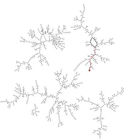
A pictorial description of the rho method can be given by drawing the Greek letter ρ representing the random walk and starting at the tail at P0. “Walking” along the line means going from Pi to Pi+1. If a collision occurs at Pt, then Pt =Pt+s for some integer s, and the elementsPt, Pt+1, . . . , Pt+s−1 form a loop. See Figure 1, and see Figure 2 for an example of how this picture occurs inside the complete graph of a function.
In the original paper by Pollard it is proposed to find a collision with Floyd’s cycle-finding algorithm. The idea of this algorithm is to walk along the sequence at two different speeds and wait for a collision. This is usually realized by using the two sequencesPi and P2i. Doing a step means to increasei by 1. IfPi =P2i for some i, then we have found a collision.
• •
• •
•
•
•
• •
P0
P1
P2
Pt−1
Pt
Pt+1
Pt+2
Pt+s−2
Pt+s−1
Pt+s
Fig. 1. Abstract diagram of the rho method.
random cj and dj, is associated to each partition and the iteration function is defined as
Pi+1 =f(Pi) =Pi⊕Rψ(Pi),
and the values ofai andbi are updated asai+1 =ai+cj, bi+1 =bi+dj. When a collision Pq =Pm for q 6=m is found, then we obtain
[aq]P ⊕[bq]Q= [am]P ⊕[bm]Q,
which implies (aq−am)P = (bm−bq)Q and hence k = logP(Q) =
aq−am
bm−bq. This
solves the discrete-logarithm problem. With negligible probability the difference bm−bq = 0; in this case the computation has to be restarted with a different starting point P0. Teske showed that choosing r = 20 and random values for the cj and dj approximates a random walk sufficiently well for the purpose of analyzing the function. For implementations, a power of 2 such as r = 8 or r= 16 or r = 32 is more practical.
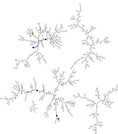
3.2 Parallelized version and distinguished points
Each instance starts at a new linear combination [a0]P⊕[b0]Qand performs the random walk until a distinguished point is found. The distinguished point, together with the coefficients ai, bi that lead to it, is then stored on a central server. The server checks for collisions within the set of distinguished points and can solve the DLP once one collision is found. As before, the difference bm−bq can be zero. In this case the distinguished point Pq is discarded and the search continues; note that the other stored distinguished points can lead to collisions since all processes are started independently at random.
See Figure 3 for an illustration of the distinguished-points method.
4
Automorphisms of small order
Elliptic-curve groups allow very fast negation. On binary curves such as the Certicom challenge curves, the negative of P = (x, y) is −P = (x, y+x). One can speed up the rho method by a factor of √2 (cf. [WZ98]) by choosing an iteration function defined on sets {P,−P}. For example, one can take any iter-ation function g, and define f(x, y) as g(min{(x, y),(x, y+x)}), ensuring that f(−P) =f(P). Here min means lexicographic minimum. Special care has to be taken to avoid fruitless short cycles; see method 1 below for details.
The ECC2-131 challenge has group size n ≈ 2130; up to negation there are n/2≈ 2129 sets {P,−P}. In this case the expected number of steps is approxi-matelypπn/4≈264.8. The ECC2-163 challenge has group sizen≈2162; in this case pπn/4≈280.8.
The ECC2K-130 challenge has group size n≈ 2129. The DLP is easier than for the ECC2-131 challenge because this curve is a Koblitz curve allowing a very fast Frobenius endomorphism. Specifically, if (x, y) is on the ECC2K-130 curve then σ(x, y) = (x2, y2), σ4(x, y) = (x4, y4) and so on through (x2130
, y2130
) are on the ECC2K-130 curve; note that (x2131
, y2131
) = (x, y). One can speed up the rho method by an additional factor of √131 by choosing an iteration function defined on sets ±σi(x, y)|0≤i < n ; there are only about n/262 ≈ 2121 of these sets. In this case the expected number of rho iterations is approximately p
πn/524≈260.8. Similarly, the expected number of iterations for the ECC2K-163 challenge is approximately 277.2.
The remainder of this section focuses on Koblitz curves, i.e. curves defined overF2 that are considered over extension fieldsF2n and considers how to define
walks on classes under the Frobenius endomorphism.
4.1 Method 1
This method was discovered by Wiener and Zuccherato [WZ98] and Gallant, Lambert, and Vanstone [GLV00]. To apply the parallel Pollard rho method, the iteration function (or step function) in the first method uses ar-adding walk (see [Tes01]), i.e. we haver pre-defined random pointsR0, . . . , Rr−1 on the curve. To perform a step of the walk, we add one of the Rj’s to the current point Pi to obtain Pi+1. To determine which point to add to Pi, we partition the group of points on the curve into r sets and define the map
ψ:E(F2n)7→ {0, . . . , r−1}, (1)
which assigns to each point on the curve one of the r partitions. With this map, we could define the walk and the iteration function f as follows:
Pi+1 =f(Pi) =Pi⊕Rψ(Pi). (2)
However, more care is required to avoid fruitless, short cycles. Assume thatPi is such that the unique representative of the class ofPi+1 =Pi⊕Rψ(Pi) is −Pi+1;
this happens with probability 1/(2n). With probability 1/rthe next added point Rψ(−Pi+1) equals Rψ(Pi) and thus Pi+2 = Pi and the walk will never leave this cycle. The probability of such cycles is 1/(2rn) and is thereby rather high. See [WZ98] for a method to detect and deal with such cycles.
We define the unique representative per class by lexicographically ordering allx-coordinates of the points in the class and choosing the “smallest” element in that order. This element has most zeros starting from the most significant bit. Of the two possibley-coordinates chose the one with lexicographically smaller value. Given that y andy+xare the candidate values and that the number of leading zeros ofx is known already, say i, it is easy to grab the distinguishing bit in the y-coordinate as the (i+ 1)-th bit starting from the most significant bit. LetΦ(P) be this unique representative of the class containing P and let (b4, b3, b2, b1,1) be the five least significant bits of Φ(P). Let j = (b4, b3, b2, b1)2. Then we can define the value of ψ(P) to be j ∈ {0, . . . ,15}. The iteration function is then given by
Pi+1 =f(Pi) =Φ(Pi)⊕Rψ(Pi).
To parallelize Pollard rho, we also need to define distinguished points (or rather distinguished classes in the present case). For each class, we use the m most significant bits of x(Φ(P)). If these bits are all zero, then we define this point (class) to be a distinguished one. With this, we can apply the methods from Section 3.
4.2 Method 2
This method does not need any precomputed random pointsRi on the curve. Instead, we define the walk and the iteration function f as
Pi+1 =f(Pi) =Pi⊕σj(Pi), (3) where j is the Hamming weight of the binary representation of x(Pi) in normal basis representation and σ the Frobenius automorphism. Note that if the com-putations are not carried out in normal-basis representation it is necessary to change the representation ofx(P) from polynomial basis to normal basis at ev-ery step. Note that in normal-basis representation the Hamming weight ofx(Pi) is equal to the Hamming weight ofx(±σk(Pi)) for all k∈ {0, . . . ,130}. Note also that
±σ(Pi+1) =±σ(Pi)±σj(σ(P)) =f(±σ(P)) and thus the step function is well defined on the classes.
For parallel Pollard rho, we also need to define distinguished points (classes). For example, we can say that a class is a distinguished one if the Hamming weight of x(P) is less than or equal to w for some fixed value of w. Note that the value ofa determines the parity of the Hamming weight since for all points Tr(x(P)) = Tr(a). This means that ( wn+ w−2n +· · ·)/2n−1 approximates the probability of distinguished points as only about 2n−1 different values can occur as x-coordinates.
The proposed version by Gallant, Lambert, and Vanstone [GLV00] does not use the Hamming weight to define j. Instead they use a unique representative per class, e.g. the point with lexicographically smallest x-coordinate, and put j = hash(x(P)) for hash a hash function from F2n to {0,1, . . . , n−1}. Using
the Hamming weight of x(P) instead avoids the computation of the unique representative at the expense of a somewhat less random walk. There are many more points with a Hamming weight around n/2 than there are around the extremal values 0 andn−1. See Section 6.2 for analysis of the loss of randomness. Harley included an extra tweak to method 2 by using the Hamming weight for updating the points but restricting the maximal exponent of σ in
Pi+1 =f(Pi) =Pi⊕σ¯j(Pi), (4) by taking ¯j as essentially the remainder of j modulo 7. He observed that for n = 109 the equality (1 +σ3) = −(1 +σ) holds. He settled for scalars (1 + σ1),(1 +σ2),(1 +σ4),(1 +σ5),(1 +σ6),(1 +σ7), and (1 +σ8). This limits the number of timesσ has to be applied per step. For sizes larger than 109 somewhat larger exponents should be used. The walks resulting from this method are even less resembling random walks but the computation is sped up by requiring fewer squarings.
5
Cost estimates
estimates to the different computation platforms we use in our attack. The fine tuning for the Certicom challenge ECC2K-130 is given in Section 6. In the fol-lowing we use I to denote the cost of a field inversion, M to denote the cost of a field multiplication, andS to denote the cost of a field squaring.
5.1 Point representation and addition
Most high-speed implementations of elliptic-curve cryptography use inversion-free coordinate systems for the scalar multiplication, i.e. they use a redundant representation P = (XP :YP :ZP) to denote the affine point (XP/ZP, YP/ZP) (for ZP 6= 0). In Pollard’s rho method it is important that Pi+1 is uniquely determined by Pi. Thus we cannot use a redundant representation but have to work with affine points. For ordinary binary curves y2 +xy = x3 + ax2 + b addition of P = (xP, yP) and Q= (xQ, yQ) with xP 6=xQ is given by
(xR, yR) = (λ2+λ+a+xP +xQ, λ(xR+xP) +yP +xR), where λ= yP +yQ xP +xQ .
Each addition needs 1I, 2M, and 1S. Note that one of the multiplications could be combined with the inversion to a division. However, we use a different opti-mization to reduce the expense of the inversion, the by far most expensive field operation.
5.2 Simultaneous inversion
All machines will run multiple instances in parallel. This makes it possible to reduce the cost of the inversion by computing several inversions simultaneously using a trick due to Montgomery [Mon87]. Montgomery’s trick is easiest ex-plained by his approach to simultaneously inverting two elements a and b.
One first computes the product c = a ·b, then inverts c to d = c−1 and obtains a−1 =b·d and b−1 =a·d. The total cost is 1I and 3M instead of 2I. By extending this trick to N inputs one can obtain inverses of N elements at the cost of 1I and 3(N −1)M.
IfN processes are running in parallel on one machine and the implementation uses Montgomery’s trick to simultaneously invert allN denominators appearing in theλ’s above, the cost per addition decreases to (1/N)I, (2 + 3(N−1)/N)M, and 1S; for large N this can be approximated by 5M and 1S.
5.3 Inversion
Inversion is by far the most costly of the basic arithmetic operations. Most implementations use one of two algorithms: the Extended Euclidean Algorithm (EEA), published in many papers and books [MvOV96], [ACD+06] and Itoh-Tsujii’s method [IT88] which essentially is using Fermat’s little theorem.
Let F2n be represented in polynomial basis. Each field element f can be
u and v such that f u+ F v = 1. Then uf ≡ 1 modF, degu < n and thus u represents the multiplicative inverse of f. The classical EEA performs a full division at each step. In practice for F2n ∼= F2[X]/F(X), implementers often
choose a version of the EEA that replaces the divisions with division by X (a right shift of the operand). Although this approach requires more iterations, it is generally faster in practice. This is the approach most commonly seen when elements of F2n are represented in polynomial basis but special implementation
strategies such as bit slicing are more suited for Itoh-Tsujii.
Although variants of EEA have been developed for normal basis representa-tion [Sun06], the most efficient approach is generally based on Itoh-Tsujii. This algorithm proceeds from the observation that in F2n, f2
n
= f, f2n−1 = 1, and therefore f2n−2
= f−1. Instead of performing divisions as in EEA, this algo-rithm computes the 2(2n−1 −1)th power. If f is represented in normal basis, squarings are simply a left shift of the operand. The exponent is fixed through-out the computation, so addition chains can be used to minimize the number of multiplications. For n = 131 a minimum-length addition chain to reach 130 is 1,2,4,8,16,32,64,128,130 and the corresponding addition chain on the expo-nents is 21−1 = 1,22−1,24−1,28−1,216−1,232−1,264−1,2128−1,2130−1.
5.4 Field representation
Typically fields are represented in a polynomial basis using the isomorphism
F2n ∼=F2[z]/F(z), where F(z) is an irreducible polynomial of degree n. A basis
is given by{1, z, z2, . . . , zn−1}. In this representation addition is done component wise and multiplication is done as polynomial multiplication moduloF. Squaring is implemented as a special case of multiplication; since all mixed terms disap-pear in characteristic 2 the cost of a squaring is basically that of the reduction moduloF. The Certicom challenges (see Section 2) are given in polynomial-basis representation with F an irreducible trinomial or pentanomial.
An alternative representation of finite fields is to use normal bases. A normal basis is a basis of the form {θ, θ2, θ22, . . . , θ2n−1
} for some θ ∈ F2n. Also in
this representation addition is done component wise. Squaring is very easy as it corresponds to a cyclic shift of the coefficient vector: ifc=Pni=0ciθ2
i
then c2 = Pn
i=0ciθ2
i+1
= Pni=0ci−1θ2
i
, where c−1 = cn. Multiplications are significantly more complicated — to expressθ2i+2j in the basis usually a multiplication matrix is given explicitly. If this matrix has particularly few entries then multiplications are faster. The minimal number is 2n−1; bases achieving this number are called optimal normal bases. For n = 131 such a basis exists but for n = 163 it does not. Alternatives are to use Gauss periods and redundant representations to represent field elements.
5.5 Cost of one step
In the following sections we will consider implementations on various platforms in different representations — in particular looking at polynomial and normal basis representations. When using distinguished points within the random walk it is important that the walk is defined with respect to a fixed field representation. So, if different platforms decide to use different representations it is important to change between bases to find the next step.
The following sections collect the raw data for the cost of one step, in Sec-tion 6 we go into details of how the attack against ECC2K-130 is implemented and give justification.
For the Koblitz curves when using method 1, each step takes 1 elliptic curve addition, (n−1)S (to find the lexicographically smallest representative), and 1S
to a variable power of they-coordinate. In particular ifx(P)2m
gave the unique representative, one needs to computey(P)2m. Note that the intermediate powers ofy(P) are not needed and special routines can be implemented. We report these figures asm-squarings, costing mS. We do not count the costs for updating the counters ai andbi.
When using method 2 each step takes 1 elliptic curve addition and 2 mS. If the computations are done in polynomial basis, then also the cost for conversion to normal basis need to be considered. If Harley’s speedup is used, then the m in them-squarings is significantly restricted.
6
Fine-tuning of the attack for Certicom ECC2K-130
In this section, we describe the concrete approach we take to attack the DLP on ECC2K-130 defined in Section 2.
6.1 Choice of step function
Of course we use the Frobenius endomorphism and define the walk on classes under Frobenius and negation. Of the two methods described in Section 4 we prefer the second. Advantages are that it can be applied in polynomial basis as well as in normal basis, that it automatically avoids short, fruitless cycles and thus does not require special routines, that there is no need to store pre-computed points, and that it avoids computing the unique representative in the step function (computing the Hamming weight is faster than 130S). If the main computation is done in polynomial-basis representation, a conversion to normal basis is required.
logarithms of (1 +σj) modulo ℓ. The shortest vector in the lattice spanned by the logarithms has four-digit coefficients. This means that fruitless collisions are highly unlikely.
6.2 Heuristic analysis of non-randomness
Consider an adding walk on ℓ group elements that maps P to P +R0 with probability p0, P +R1 with probability p1, and so on through P +Rr−1 with probability pr−1, where R0, R1, . . . , Rr−1 are distinct group elements and p0+ p1+· · ·+pr−1 = 1.
IfQis a group element, andP, P′are two independent uniform random group elements, then the probability thatP, P′ both map toQwithout havingP =P′ is (1−p2
0−p21−· · ·−p2r−1)/ℓ2. Indeed, ifP =Q−Ri andP′ =Q−Rj, withi6=j, thenP maps toQwith probabilitypiandP′maps toQwith probabilitypj; there is chance 1/ℓ2 that P =Q−Ri and P′ =Q−Rj in the first place; overall the probability is Pi6=jpipj/ℓ2 = (Pi,jpipj−Pjp2j)/ℓ2 = (1−
P
jp2j)/ℓ2. Adding over the ℓ choices of Q one sees that the probability of an immediate collision from P, P′ is at least (1−P
jp2j)/ℓ.
In the context of Pollard’s rho algorithm (or its parallelized version), after a total of T iterations, there are T(T − 1)/2 pairs of iteration outputs. The inputs are not uniform random group elements, and the pairs are not indepen-dent, but one might nevertheless guess that the overall success probability is approximately 1−(1−(1−Pjp2j)/ℓ)T(T−1)/2, and that the average number of iterations before success is approximatelyqπℓ/(2(1−Pjp2
j)). This is a special case of the variance heuristic introduced by Brent and Pollard in [BP81].
For example, if p0 =p1 =· · · =pr−1 = 1/r, then this heuristic states that ℓ is effectively divided by 1−1/r, increasing the number of iterations by a factor of 1/p1−1/r≈1 + 1/(2r), as discussed by Teske [Tes01].
The same heuristic applies to a multiplicative walk that mapsP tosjP with probabilitypj: the number of iterations is multiplied by 1/
q
1−Pjp2
j. In par-ticular, for the ECC2K-130 challenge, the Hamming weight ofx(P) is congruent to 0,2,4,6,8,10,12,14 modulo 16 with respective probabilities approximately
0.1443,0.1359,0.1212,0.1086,0.1057,0.1141,0.1288,0.1414,
so our walk multiplies the number of iterations by approximately 1.069993. Note that any walk determined by the Hamming weight will multiply the number of iterations by at least 1/
q
1−Pj 1312j2/2260≈1.053211.
6.3 Choice of distinguished points
since ( 13128+ 13126+· · ·)/2130is approximately 2−35.4, and an expected number of 225.5 distinguished points. Note that for this curve a = 0 and thus each x-coordinate has trace 0 and so the Hamming weight is even for any point. If we instead choose Hamming weight 32 for distinguished points then there will be an average length of 228.4 steps before hitting a distinguished point and an expected number of 232.5 distinguished points.
6.4 Implementation details
Most computations will not lead to a collision. Our implementation does not compute the intermediate scalars ai and bi nor does it store a list of how often each of the exponents j appeared. Instead the starting point of each walk is computed deterministically from a saltS. When a distinguished point is found, the salt together with the distinguished point is reported to the central server.
When distinguished points are noticed, x(P) is given in normal basis rep-resentation, so it makes sense to keep them in normal basis. To search for col-lisions it is necessary to have a unique representative per class. We choose the lexicographically smallest value of x(P), x(P)2, . . . , x(P)2130. In normal basis representation this is easily done by inspecting all cyclic shifts ofx(P). To save bandwidth a 64-bit hash of this unique representative is reported to the server along with the original 64-bit seed.
If the server detects a collision on the 64-bit hash, it recovers the two starting points from the salt values and follows the random walk from the initial points, this time keeping track of how often each of the powersj appears. Like in the ini-tial computation the distinguished point is noticed by a small Hamming weight of the normal basis representation of the x-coordinate. If the x-coordinates co-incide up to cyclic shifts, i.e. the partial collision gave rise to a complete one, the unique representative per class is computed. Note that this time also the y-coordinate needs to be transformed to normal basis to obtain the correct result. Finally the equivalence of σ and smodℓ is used to compute the scalars on both sides and thereby (eventually) the DLPP(Q).
It is possible for a 64-bit hash collision to occur by accident, rather than from a distinguished-point collision. We could increase the 64-bit hash to 96 bits or 128 bits to eliminate these accidents. However, a larger hash costs bandwidth and server storage, and the benefit is small. Even with as many as 232 distinguished points, accidental 64-bit collisions are unlikely to occur more than a few times, and disposing of the accidents has negligible cost.
7
FPGA implementations
The attacks presented in this section are developed for the latest version of CO-PACOBANA [KPP+06], which is a tightly integrated, reconfigurable hardware cluster.
The 2009 version of COPACOBANA offers 128 Xilinx Spartan-3 XC3S5000-4FG676 FPGAs, laid out on 16 plug-in modules each hosting 8 chips. Each chip is configured with 32 MB of dedicated off-chip local RAM. Serial data lines connect the FPGAs as a systolic array on the backplane, passing data packets from one device to the next in round robin fashion before they finally reach their destination. Up to two separate controller units interface the systolic array (via PCIe) to the mainboard of a low-profile PC that is integrated within the same case as COPACOBANA. In addition to data routing, the PC can perform post-processing before it stores or distributes the results to other nodes.
This section presents preliminary results comparing two choices for the un-derlying field arithmetic on COPACOBANA. The first approach performs arith-metic operations on elements represented in polynomial basis, converting to nor-mal basis as needed, while the second operates directly on elements represented in normal basis.
7.1 Polynomial basis implementation
The cycle counts and delay are based on the results of implementations on FPGA (Xilinx XC3S5000-4FG676). For multiplication, digit-serial multiplier is imple-mented. The choice of digit-size is based on a preliminary exploration of the trade-off between speed and area. Here we choose digit-size d = 22 and d = 24 for F2131 and F2163, respectively.
For inversion, we used the Itoh-Tsujii algorithm. Although EEA runs faster than Itoh-Tsujii, it requires its own data path, adding extra cost in area. Using Montgomery’s trick for batch inversion lowers the amortized cost to (3−1/N)M+ (1/N)Iper inversion. The selection ofN = 64 is a trade-off between performance and area. One inversion in F2131 takes 212 cycles, and one multiplication takes
8 cycles. Choosing N = 64, each inversion on average takes 28 cycles, and the whole design takes 8 out of 104 BRAMs on the target FPGA. If we increase N to 128, the cost of one inversion drops to 26 cycles. However, the whole design requires 16 BRAMs. Since the current design uses around %11 of the LUTs of the FPGA, we can put 8∼9 copies of current design onto this FPGA if we do not use more than %11 BRAMs for each.
Tab. 1 shows the cycle counts of each field operation. The cost of memory access is included.
additions squaringsm-squarings multiplications inversions batch-inv. (N = 64)
F2131 2 2 m+1 8 212 28
F2163 2 2 m+1 9 251 31
Table 1. Cycle counts for field operations in polynomial basis on XC3S5000-4FG676
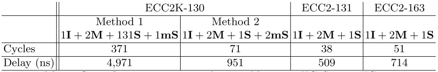
The design is synthesized with Xilinx ISE 11.1. On Xilinx XC3S5000-4fg676 FPGA, our current design for F2131 and F2163 can reach a maximum frequency
of 74.6 MHz and 74 MHz, respectively. Table 2 shows the delay of one iteration.
ECC2K-130 ECC2-131 ECC2-163
Method 1 Method 2
1I+ 2M+ 131S+ 1mS1I+ 2M+ 1S+ 2mS 1I+ 2M+ 1S1I+ 2M+ 1S
Cycles 371 71 38 51
Delay (ns) 4,971 951 509 714
Table 2.Cost of one iteration in polynomial basis on XC3S5000-4FG676
The current design for ECC2K-130 uses 3,656 slices, including 1,468 slices for multiplier, 75 slices for square, 1,206 slices for base conversion and 117 slices for Hamming Weight counting. Since a Xilinx XC3S5000 FPGA has 33,280 slices, taking input/output circuits into account, we estimate 9 copies of the polynomial-basis design can fit in one FPGA. Considering 235 iterations are re-quired on average to generate one distinguished point, each copy generates 2.6 distinguished points per day. A single chip can then be expected to yield 23.4 distinguished points per day.
The current design for ECC2-131 uses 2,206 slices. Note that circuits to search for the smallest x(P) is not included. We estimate that 12 copies (limited by BRAM) can fit in one FPGA.
The current design for ECC2K-163 uses 4,446 slices, including 2,030 slices for multiplier, 94 slices for square and 1,209 slices for base conversion and 217 slices for Hamming Weight counting. We estimate that 7 copies can fit in one FPGA.
The current design for ECC2-163 uses 3,242 slices. Note that circuits to search for the smallest x(P) is not included. We estimate that 9 copies can fit in one FPGA.
For ECC2-131, it is the number of BRAM that stops us putting more copies of ECC engine. We believe that the efficiency of BRAMs usage can be further improved, and more copies can be instantiated on one FPGA.
7.2 Normal basis implementation
digit-serial version currently under development. The bit-serial design computes a single bit of the product in each clock cycle. Because of this relatively slow performance, it consumes very little area. For F2131, the multiplier takes 466
slices of the chip’s available 66,560, or less than 1%, while F2163 requires 679
slices, or around 1%.
additions squaringsm-squarings multiplications inversions batch-inversions
F2131 1 1 1 131 1065
F2163 1 1 1 163 1629
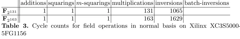
Table 3. Cycle counts for field operations in normal basis on Xilinx XC3S5000-5FG1156
An implementation of the full Rho step would instantiate at least one mul-tiplier expressly for the Itoh-Tsujii inversion routine and process several points simultaneously to keep the inversion unit busy. Our implementation results take this approach: each engine consists of one multiplier dedicated to inversion and eight for ordinary multiplication. The result for F2131 is an area requirement of
1,915 slices while achieving a clock rate of 85.898 MHz.
The inversion unit is the bottleneck at 1,065 cycles required. We can use Montgomery’s trick to perform many simultaneous inversions. So the design challenge becomes one of keeping the inversion unit busy, spreading the cost of the inverter across as many simultaneous Rho steps as possible.
Suppose we process 32 inversions simultaneously using one inversion unit. This operation introduces 8Mcycles of delay. Method 2 requires 1I+ 2M+ 1S+ 1mS to compute one step of the Rho method. Because squarings are free, we must compute two additional multiplications per step. On top of this cost are the 3(N −1) = 157 multiplications needed for the pre- and post-computation to obtain individual inverses. Although we might be able to spread a particular step across several multipliers, we can safely assume that keeping the inversion unit busy this way requires up to a total of 32 additional multipliers. The chip has embedded storage for up to 1,664 points, far more than required. With this approach, these multipliers would be idle roughly five-eighths of the time; this estimate is meant to be conservative. At a cost of 466 slices each, we can expect an engine to consume a total of 14,912 slices. Instantiating all these multipliers has the advantage that we can complete 32 steps every 1,065 cycles, or one step every 34 cycles. At 85.898 MHz, that equates to 2,526,411 steps per second, or 6 distinguished points per day per engine. As a single chip has 66,360 slices available, four of these engines could be instantiated per chip, yielding 24 distinguished points per day per chip. This figure may underestimate the time required for overhead like memory access.
at a cost of additional area. We are currently implementing this approach; the previous work indicates that this approach can improve the time-area product.
As of this writing, normal-basis results for F2163 are still pending.
7.3 Comparison
Both polynomial and normal-basis implementations offer roughly the same per-formance today. Because the polynomial-basis implementation is in a more ma-ture state, embodying the entire step of the Rho method, it represents less risk and uncertainty in terms of use in a practical attack. It achieves this performance despite the fact that this particular Certicom challenge would appear to be ide-ally suited to a normal-basis implementation. As a case in point, the polynomial version must pay the overhead to convert elements back to normal basis at the end of each step to check if a distinguished point has been reached.
As this paper represents work in progress, the normal-basis figures in this section are based on measurements only of the field arithmetic time and area. While the estimates may not fully account for overhead like memory access, they also do not capture the effect of migrating to a digit-serial multiplier. Because multiplication cost dominates the cost of inversion – and therefore the cost of a step of the Rho method, the normal-basis approach may ultimately offer higher performance because in this particular attack. Performance of the polynomial-basis version may also improve in unforeseen ways and it would undoubtedly outperform the normal-basis version in an attack on ECC2-131.
8
Hardware implementations
In this section we present and discuss the results achieved while targeting ASIC platforms. To obtain the estimates presented in this work, we have used the UMC L90 CMOS technology, using the Free Standard Cell library from Fara-day Technology Corporation characterized for HS-RVT (high speed regular Vt) process option with 8 Metal layers. For synthesis results we have used design compiler 2008.09 from Synopsys, and for placement and routing we have used SoC Encounter 7.1-usr3 from Cadence Design Systems.
Both synthesis and post-layout analysis use typical corner values, and rea-sonable assumptions for constraints. The designs are for performance estimate and are not refined for actual production (i.e. they do not contain test struc-tures, a practical I/O subsystem). During synthesis, multiple runs were made with different constraints, and the results with the best area time product have been selected.
8.1 Polynomial basis implementation
Addition The addition of n-bits will always be equal to 2n-input XOR gates. No separate synthesis has been made for this circuit. In a practical circuit the interconnection between the adder the rest of the circuit would have a significant impact upon the delay and the area of the circuit. The delay for the addition is approximately 75ps, while the required area is approximately n·2.5 Gate Equivalents (GEs). No post-layout results are given for this circuit as a standalone implementation is not representative.
Squaring Squaring is performed with a parallel squarer. This operator is rel-atively inexpensive thanks to the use of a sparse irreducible polynomial, a pentanomial, which is hardwired. Each bit of the result is therefore com-puted using few XOR gates. The detailed results for ASIC implementation are reported in Table 4, where, due to the small size of this component, no post-layout analysis is provided.
F2131 F2163
Pre-layout Pre-layout
Delay (ps) ∼ 250 250
Frequency (GHz) ∼ 4.0 4.0
Flip-Flop Number 131 163
Area (mm2
) ∼ 0.003 0.004
GE ∼ 960 1200
Table 4.Results for ASIC implementation of Squarer in polynomial basis
m-Squaring This operation can be implemented using a single squarer that iteratively computes the m squarings inm clock cycles.
Multiplication In order to perform the modular multiplication, we used a sub-quadratic Karatsuba parallel multiplier. As for squaring, the modular reduc-tion step is easily performed with a few XOR gates for each bit of the result. The modular multiplier has a pipeline depth of 8 clock cycles in both F2131
and F2163 and produces a result at each clock cycle. The detailed results for
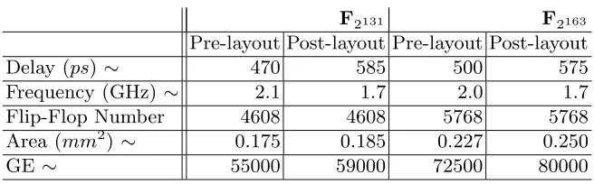
the modular multiplication are reported in Table 5
F2131 F2163
Pre-layout Post-layout Pre-layout Post-layout
Delay (ps) ∼ 470 585 500 575
Frequency (GHz)∼ 2.1 1.7 2.0 1.7
Flip-Flop Number 4608 4608 5768 5768
Area (mm2
) ∼ 0.175 0.185 0.227 0.250
GE∼ 55000 59000 72500 80000
Inversion The inversion is based on Fermat’s little theorem with the multipli-cation chain technique by Itoh and Tsujii. This method is preferred to the extended Euclidean algorithm according to the comparison of both methods performed in the work by Bulens et al. [BMdDQ06]. An inversion requires 130 squarings and 8 multiplications in F2131 and 162 squarings and 9
multi-plications in F2163. The inverter uses the parallel multiplier described above
and a block of several pipelined consecutive squarers. This block allows to speed up the consecutive squarings required in the inversion using the Itoh-Tsujii technique. It is done by putting several squarers in a serial way, so that every bit of the result is now computed with a larger number of XOR gates, depending on the number of squarings to be performed. Within the inverter, the block of consecutive squarers actually allows to compute sev-eral possible numbers of consecutive squarings (the numbers of consecutive squarings specified by the technique of Itoh and Tsujii). The inversion is done by looping over the multiplier and the squarer according to the tech-nique of Itoh and Tsujii. For this purpose, extra shift registers are required. The inverter has a pipeline depth of 16 and achieves an inversion with a mean delay of 10 and 11 clock cycles in F2131 and F2163 respectively.
A lower bound on the area requirement of the inverter can be found by gath-ering the results for the squarer and the multiplier. This leads to around 60000 GE for F2131 and 81200 for F2163. However, this assumes an
itera-tive use of the squarer. For the parallel pipelined inverter described above, a better estimate can be obtained by approximating the block of consecu-tive squarers as a series of single squarers. The number of these consecuconsecu-tive squarers is given by the maximum number of consecutive squarings in the technique of Itoh and Tsujii on F2131 and F2163, i.e. 64 in both cases. As a
result, the area cost of the block of consecutive squarers should be around 64000 and 76800 GE forF2131 and F2163 respectively, leading to an area cost
of 123000 GE and 156800 for the full parallel inverter on F2131 and F2163
respectively.
The inverter has a much higher area cost and lower throughput with respect to the multiplier. From an area-time point of view, it is interesting to com-bine several inversions using the Montgomery trick instead of replicating several inverters when trying to increase the throughput of inversions. As each combined inversion requires 3 multiplications to be performed, it seems to be always interesting to use the Montgomery trick instead of replicating several inverters. In practice, the gain of using Montgomery’s trick can be smaller than expected, as stated in [BMdDQ06]. Simultaneous inversion does not require a specific operator as it can be built upon the multiplier and the inverter.
F2131 F2163
Pre-layout Pre-layout
Delay (ps) ∼ 410 460
Frequency (GHz) ∼ 2.4 2.15
Flip-Flop Number 0 0
Area (mm2
) ∼ 0.044 0.061
GE ∼ 13900 19400
Table 6. Results for ASIC implementation of Polynomial to Normal Basis converter
additions squarings m-squarings multiplications inversions
F2131 1 1 m 1 10
F2163 1 1 m 1 11
Table 7.Cycle counts for field operations in polynomial basis on ASIC
8.2 Normal basis implementation
Addition For ASIC, the addition is performed in a way similar to the one of polynomial bases.
Squaring In normal basis, the squaring is equivalent to a rotation, thus the impact on the area and delay of this component will be mainly due to the interconnections.
m-Squaring This operation can be achieved by an iterative use of a single squarer as for the polynomial basis. However, since a squaring is equivalent to a rotation, one can anticipate themrotations and perform this operation in one clock cycle.
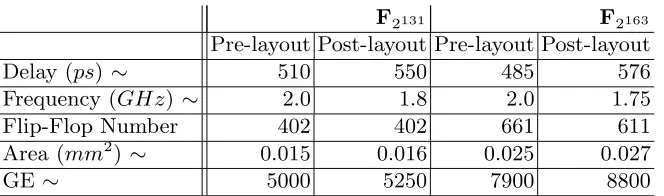
Multiplication The proposed implementation is based on a bit-serial multiplier which calculates a single bit product every clock cycle. The detailed results for the modular multiplication are reported in Table 8.
F2131 F2163
Pre-layout Post-layout Pre-layout Post-layout
Delay (ps) ∼ 510 550 485 576
Frequency (GHz) ∼ 2.0 1.8 2.0 1.75
Flip-Flop Number 402 402 661 611
Area (mm2
) ∼ 0.015 0.016 0.025 0.027
GE ∼ 5000 5250 7900 8800
Table 8.Results for ASIC implementation of Field element multiplier in normal basis
should not be significantly higher than the cost of the multiplier since the multiple squarings can be performed with interconnections only. Therefore, it should be close to the lower bound given by the area cost of the multiplier, i.e. 5250 GE for F2131.
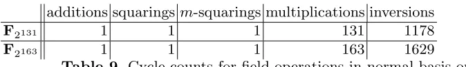
additions squaringsm-squarings multiplications inversions
F2131 1 1 1 131 1178
F2163 1 1 1 163 1629
Table 9. Cycle counts for field operations in normal basis on ASIC
8.3 Cost of step on ECC2K-130
A step in the Pollard rho computation on ECC2K-130 consumes 1I+2M+131S+ 1mSusing method 1. In polynomial basis, this takes 273 cycles on an ASIC while in normal basis it takes 1572 cycles. Using method 2, a step requires 1I+ 2M+ 1S+ 2mS and the additional conversion to normal basis if the computations are done in polynomial basis. In polynomial basis, the step is performed in 274 cycles on an ASIC while in normal basis it is done in 1443 cycles. A larger cycle count for the normal basis is due to the iterative approach of the design of the components in this basis as opposed to the parallel design used for the polynomial basis. These cycles counts do not consider the use of simultaneous inversion since the gain of this method should be assessed once the whole processor is assembled, following [BMdDQ06]. This technique should be employed as much as possible given the high cost of an inversion. Therefore, the cycle counts are likely to be significantly lower in practice. For instance, combining 10 inversions theoretically lowers the cycle count for the step in normal basis by about 50%.
Concerning the area, a lower bound can be determined by gathering the costs of the operators. Note that this bound does not include the cost of storing elements. In polynomial basis, the lower bound on the area of a processor based on the components described above is roughly 125000 GE when using method 1 and 140000 GE for method 2. It is mostly the cost of the inverter, as its multiplier can also be used to perform the two multiplications needed in each step. In normal basis, the same estimate leads to 6000 GE (mainly the cost of the multiplier). Based on these estimates, the processor relying on the normal basis appears to be more efficient from an area-time point of view as it is roughly 6 times slower but 20 times smaller. However, the use of several squarers in parallel should improve the area-time product of the processor relying on the polynomial basis.
8.4 Cost of step on ECC2-131
1441 cycles. Again, the iterative approach used in the normal basis causes a higher cycle count for the normal basis operators. The area costs are on the same order as on ECC2K-130. Therefore, the processor based on the polynomial basis appears to be more efficient here since it is 110 faster while being only 20 times larger.
8.5 Cost of step on ECC2-163
A step in the Pollard rho computation on ECC2-163 consumes 1I+ 2M+ 1S. In polynomial basis this takes 14 cycles on ASIC while in normal basis it takes 1956 cycles.
The processor based on the polynomial basis has a lower bound on the area cost around 160000 GE (mainly the cost of the inverter). It is 140 times faster than the one based on the normal basis. For this reason, it is expected to be more area-time efficient, as on ECC2-131.
8.6 Detailed cost of the full attack on ECC2K-130
With the cost of individual arithmetic blocks given above, we can now attempt a first order estimation of cost and performance of an ASIC that could be used for the ECC2K-130 challenge. We will consider using a standard 16mm2 die in the 90nm CMOS technology using a multi-project wafer (MPW) production in prototype quantities. The cost of producing and packaging 50-250 of such ASICs is estimated to be less than 60 000 EUR.
The performance of the subcomponents described in the preceding sections were all post-layout figures that include interconnection delays, clock distribution overhead and all required registers. We estimate that the overall clock rate will be around 1.5 GHz when all the components are combined into one system. Each chip would require a PLL for to distribute the internal clock. In this estimation we will again leave a generous margin in the timing and will assume that the system clock is 1.25 GHz.
9
AMD64 implementations
This section describes our software implementation for general-purpose CPUs supporting the amd64 (also known as “x86-64”) instruction set. This imple-mentation is tuned for Intel’s popular Core 2 series of CPUs but also performs reasonably well on other recent CPUs, such as the AMD Phenom.
9.1 Bitslicing
New speed records for elliptic-curve cryptography on the Core 2 were recently announced in a Crypto 2009 paper [Ber09a]. The new speed records combine a fast complete addition law for binary Edwards curves, fast bitsliced multipli-cation for arithmetic in F2n, and the Core 2’s fast instructions for arithmetic
on 128-bit vectors. Our amd64 implementation combines the bitsliced multipli-cation techniques from [Ber09a] with several additional techniques for bitsliced computation. (Binary Edwards curves do not appear to save time in this context; the implementation uses standard affine coordinates for Weierstrass curves.)
Bitslicing a data structure is a simple matter of transposition. Our imple-mentation represents 128 elliptic-curve points (x0, y0),(x1, y1), . . . ,(x127, y127), with xi, yi ∈ F2n, as 2n vectors X0, X1, . . . , Xn−1, Y0, Y1, . . . , Yn−1, where the
jth bits of Xi and Yi are the ith bits of xj andyj respectively.
“Logical” vector operations act on bitsliced inputs as 128-way SIMD instruc-tions. For example, a vector XOR carries out xors in parallel on 128 pairs of bits. Multiplication in F2n can be decomposed into bit operations, a series of
bit XORs and bit ANDs; one can carry out 128 multiplications on 128 pairs of bitsliced inputs in parallel by performing the same series of vector XORs and vector ANDs. XOR and AND are not the only operations available, but other operations do not seem helpful for multiplication, which takes most of the time in this implementation.
Similar comments apply to higher-level computations, such as elliptic-curve arithmetic over F2n. There is an obvious analogy between designing bitsliced
software and designing ASICs, but one should not push the analogy too far: there are fundamental differences in gate costs, communication costs, etc.
Many common software-implementation techniques for F2n arithmetic, such
as precomputed multiplication tables, perform quite badly when expressed as bit operations. However, bitslicing allows free shifts, masks, etc., and fast bit-sliced algorithms for binary-field arithmetic outperform all known non-bitbit-sliced algorithms.
9.2 Results
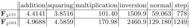
addition squaring multiplication inversion normal step
F2131 3.5625 2.6406 85.32 1089.4 103.84 694
F2163 4.0625 2.9141 140.35 1757.18 157.58 1059
Table 10. Cycle counts per input for bitsliced field operations in polynomial basis on a 3000MHz Core 2 Q6850 6fb
addition squaring multiplication inversion normal step
F2131 4.4141 3.8516 101.40 1509.9 59.063 778
F2163 4.9688 4.5859 170.98 2460.9 129.180 1249
Table 11. Cycle counts per input for bitsliced field operations in polynomial basis on a 2200MHz Phenom 9550 100f23
squarings are not the main operation in this implementation.) The implementa-tion batches 48I into 1I+ 141M, and then computes 1I as 8M+ 130S (in the case of ECC2K-130), so on average each inversion costs 3.10417M+ 2.70833S. The total cost of field arithmetic in a step is therefore 5.10417M+ 23.70833S. The “step” cycle count shown above includes more than field arithmetic:
• About 63% of the time (on a Core 2) is spent on multiplications.
• About 15% of the time is spent on conversion to normal-basis representation. This computation uses the algorithm described in [Ber09b].
• About 9% of the time is spent on squarings.
• About 7% of the time is spent on additions.
• About 3% of the time is spent on weight calculation. This calculation com-bines standard full-adder circuits in an obvious way, adding (for example) 15 bits by first adding 7 bits, then adding 7 more bits, then adding the two sums to the remaining bit.
• The remaining 3% of the time is spent on miscellaneous overhead.
The 48 inversions are actually 48 bitsliced inversions of 48·128 field elements, each containing n bits. The implementation handles 48·128 points (x, y) in parallel. Eachx-coordinate (in batches of 128) is converted to normal-basis rep-resentation, compressed to a Hamming weight, checked for being distinguished, and then further compressed to three bits that determine the point (x′, y′) that will be added to (x, y). The implementation computes eachx′by repeated squar-ing, storesx′+x along with (x, y), and inverts x′+x. The total active memory for allx, y, x′+x,1/(x′+x) is 4·48·128 field elements, together occupying 3072n bytes: i.e., 402432 bytes for n = 131, or 500736 bytes for n = 163. Subsequent elliptic-curve operations use only a few extra field elements.
10
Cell implementations
Processing Element (PPE), which can offload work to the eight Synergistic Pro-cessing Elements (SPEs) [TCC+05]. Each SPE consists of a Synergistic Pro-cessing Unit (SPU), 256 kilobytes of private memory called Local Store (LS), a Memory Flow Controller, and a register file containing 128 registers of 128 bits each. The SPUs are the target of our Cell implementation and allow 128-bit wide single instruction, multiple data (SIMD) operations. The SPUs are asymmetric processors, having two pipelines (denoted by the odd and the even pipeline) which are designed to execute two disjoint sets of instructions. Hence, in the ideal case, two instructions can be dispatched per cycle.
All performance measurements for the Cell stated in this section are obtained by running on a single SPE on a PlayStation 3 (PS3) video game console on which the programmer has access to six SPEs.
Like the amd64 architecture, the SPU supports bit-logical operations on 128-bit registers. Hence, a 128-bitsliced implementation — similar to the one presented in Section 9 — seems to be a good approach. However, for two reasons it is much harder to achieve good performance with the same techniques on the SPU:
The first reason is the restricted local storage size of only 256 KB. As bitsliced implementations work on 128 inputs in parallel, they need much more memory for intermediate values than a non-bitsliced implementation. Even if the code and intermediate results fit into 256 KB, the batch size for Montgomery inversions has to be smaller yielding a higher number of costly inversions per iteration. The second reason is that all instructions are executed in order; a fast implementation requires loop unrolling in several functions increasing the code size and limiting the available storage for batching even further.
We decided to implement both a bitsliced version and a non-bitsliced version to compare which approach gives better results for the SPE. Both implementa-tions required hand-optimizing the code on the assembly level, the main focus is on the ECC2K-130 challenge.
10.1 Non-bitsliced implementation
We decided to represent 131-bit polynomials using two 128-bit vectors. Let A, B ∈ F2131 in polynomial basis. In order to use 128-bit look-up tables and
to get 16-bit aligned intermediate results the multiplication is broken into parts as follows
A =Al+Ah ·z128 =Ael+Aeh·z121 B =Bl+Bh·z128=Bel+Beh·z15
C = A·B=Ael·Bl+Ael·Bh·z128+Aeh·Bel·z121+Aeh·Beh·z136
number of cycles. The inversion is implemented using a sequence of squarings, m-squarings and multiplications.
The optimal number of concurrent walks is as large as possible, i.e. such that the executable and all the required memory fit in the LS. In practice 256 walks are processed in parallel.
addition squaringm-squaring multiplication inversion normal step
F2131 1 - 2 38 96 149 8000 96 1157
Table 12.Cycle counts per input for non-bitsliced field operations in polynomial basis on one SPE of a 3192 MHz Cell Broadband Engine, rev. 5.1
Cost of step on ECC2K-130 A step in the Pollard rho computation on
ECC2K-130 consumes 2561 I+ 5M+ 1S+ 2mS plus the conversion from poly-nomial to normal basis when using method 2 as described in Section 4.2. The required number of cycles for one iteration on the curve ECC2K-130 are stated in Table 12. Addition is done by two XOR instructions, which go in the even pipeline, and requires at most two and at least one instruction if interleaved with two odd instructions. There are 55 miscellaneous cycles which include the additions, the calculation of the weight, the test if a point is distinguished and various overhead. The cycle counts stated in Table 12 are obtained by “count-ing” the required number of cycles of our assembly code with the help of the SPU timing tool: a static timing analysis tool available for the Cell.
10.2 Bitsliced implementation
The bitsliced implementation is based on the C++-code for the amd64 architec-ture. In a first step we ported the code to C, to reduce the size of the resulting binary. For the ECC2K-130 we then implemented bitsliced versions of multipli-cation, reduction, squaring, addition and conditional move (cmov) in assembly to accelerate the computations.
The maximal batch size that we can use for the ECC2K-130 challenge is 14. Timings for the implementation are given in Table 13, all timings include costs for function calls, they ignore costs for reading the input, which is negligible for long computations until a distinguished point has been found. The measurements are averages across billions of steps measured at runtime.
addition cmov squaring multiplication inversion normal step
F2131 5.8438 6.3125 4.5859 127.5938 1845.3125 30.7734 1046.8359
Table 13. Cycle counts per input for bitsliced field operations in polynomial basis on one SPE of a 3192 MHz Cell Broadband Engine, rev. 5.1
• About 60% of the time is spent on multiplications.
• About 3% of the time is spent on conversion to normal-basis representation.
• About 12% of the time is spent on squarings.
• About 3% of the time is spent on additions.
• About 3% of the time is spent on conditional moves.
• About 11% of the time is spent on weight calculation.
• The remaining 8% of the time is spent on miscellaneous overhead. For algorithmic details see also Section 9.
11
Complete implementation of the attack
Eventually all platforms described so far will be used to attack ECC2K-130. As a proof of concept and as infrastructure for our optimized implementations we builtref-ntl, a C++ reference implementation of an ECC2K discrete-logarithm attack using Shoup’s NTL for field arithmetic. The implementation has several components:
• Descriptions of several different ECC2K challenges that the user can target. Similarly to the data in Section 2 each description consists of an irreducible polynomial F, curve parameters a, b, curve points P, Q in hexadecimal, the order ℓ of P, the root s of T2+ (−1)aT + 2 modulo ℓ that corresponds to the Frobenius endomorphism (so thatσ(P) = [s]P), a choice of normal-basis generator, and a choice of weight defining distinguished points.
• A setup program that converts a series of 64-bit seedst1, t2, . . .into a series of curve points A(t1)P ⊕Q, A(t2)P ⊕Q, . . .. The function A uses AES to expand each seed tj into a bit-string (cj,127, cj,126, . . . , cj,1, cj,0) of length 128 and then interprets it as a Frobenius expansion to compute starting point Q⊕P127i=0cj,iσi(P).
• An iterate program that given an elliptic curve point iterates the step function until a distinguished point is found and then reports it to a server. This computation is the real bottleneck in the implementation; the task of the optimized implementations in Sections 7–10 is to perform the same computation as quickly as possible on various platforms.
• A short script that normalizes each distinguished point and sorts the nor-malized distinguished points to find collisions.
the need for the optimized implementations to keep track of the iteration steps.
• Final programs finish and verify that express each of the colliding nor-malized distinguished points as linear combinations of P and Q and that print the discrete logarithm of Q base P.
As an end-to-end test of the implementation we solved a randomly generated challenge over F241, using about one second of computation on one core of a
2.4GHz Core 2 Quad. We checked the result using the Magma computer-algebra system. We then solved ECC2K-95, as described in Section 1.
References
[ACD+
06] Roberto Avanzi, Henri Cohen, Christophe Doche, Gerhard Frey, Tanja Lange, Kim Nguyen, and Frederik Vercauteren. Handbook of Elliptic and Hyperelliptic Curve Cryptography. CRC Press, 2006.
[Ber09a] Daniel J. Bernstein. Batch binary Edwards. InCrypto 2009, volume 5677 of LNCS, pages 317–336, 2009.
[Ber09b] Daniel J. Bernstein. Optimizing linear maps modulo 2, 2009. http://cr. yp.to/papers.html#linearmod2.
[BMdDQ06] Philippe Bulens, Guerric Meurice de Dormale, and Jean-Jacques Quisquater. Hardware for Collision Search on Elliptic Curve over GF(2m
). In Proceedings of SHARCS’06, 2006. http://www.hyperelliptic.org/ tanja/SHARCS/talks06/bulens.pdf.
[BP81] Richard P. Brent and John M. Pollard. Factorization of the eighth Fermat number. Mathematics of Computation, 36:627–630, 1981.
[Cer97a] Certicom. Certicom ECC Challenge. http://www.certicom.com/images/ pdfs/cert ecc challenge.pdf, 1997.
[Cer97b] Certicom. ECC Curves List. http://www.certicom.com/index.php/ curves-list, 1997.
[GLV00] Robert P. Gallant, Robert J. Lambert, and Scott A. Vanstone. Improv-ing the parallelized Pollard lambda search on anomalous binary curves.
Mathematics of Computation, 69(232):1699–1705, 2000.
[Har] Robert Harley. Elliptic curve discrete logarithms project. http:// pauillac.inria.fr/∼harley/ecdl/.
[Har60] Bernard Harris. Probability distributions related to random mappings.
The Annals of Mathematical Statistics, 31:1045–1062, 1960.
[Hof05] H. Peter Hofstee. Power efficient processor architecture and the Cell pro-cessor. InHPCA 2005, pages 258–262. IEEE Computer Society, 2005. [IT88] Toshiya Itoh and Shigeo Tsujii. A Fast Algorithm for Computing
Mul-tiplicative Inverses in GF(2m
) Using Normal Bases. Inf. Comput., 78(3):171–177, 1988.
[KPP+
06] S. Kumar, C. Paar, J. Pelzl, G. Pfeiffer, and M. Schimmler. Breaking ciphers with COPACOBANA-a cost-optimized parallel code breaker. Lec-ture Notes in Computer Science, 4249:101, 2006.
[MdDBQ07] Guerric Meurice de Dormale, Philippe Bulens, and Jean-Jacques Quisquater. Collision Search for Elliptic Curve Discrete Logarithm over GF(2m
[Mon87] Peter L. Montgomery. Speeding the Pollard and elliptic curve methods of factorization. Mathematics of Computation, 48:243–264, 1987.
[MvOV96] A.J. Menezes, P.C. van Oorschot, and S.A. Vanstone.Handbook of Applied Cryptography. CRC Press, 1996.
[NS06] M. Novotn`y and J. Schmidt. Two Architectures of a General Digit-Serial Normal Basis Multiplier. InProceedings of 9th Euromicro Conference on Digital System Design, pages 550–553, 2006.
[Pol78] John M. Pollard. Monte Carlo methods for index computation (mod p).
Mathematics of Computation, 32:918–924, 1978.
[Sun06] Berk Sunar. A Euclidean algorithm for normal bases. Acta Applicandae Mathematicae, 93:57–74, 2006.
[TCC+
05] Osamu Takahashi, Russ Cook, Scott Cottier, Sang H. Dhong, Brian Flachs, Koji Hirairi, Atsushi Kawasumi, Hiroaki Murakami, Hiromi Noro, Hwa-Joon Oh, Shoji Onish, Juergen Pille, and Joel Silberman. The circuit design of the synergistic processor element of a Cell processor. InICCAD 2005, pages 111–117. IEEE Computer Society, 2005.
[Tes01] Edlyn Teske. On random walks for Pollard’s rho method. Mathematics of Computation, 70(234):809–825, 2001.
[vOW99] Paul C. van Oorschot and Michael J. Wiener. Parallel collision search with cryptanalytic applications. Journal of Cryptology, 12(1):1–28, 1999. [WZ98] Michael J. Wiener and Robert J. Zuccherato. Faster attacks on elliptic
curve cryptosystems. In Selected Areas in Cryptography, volume 1556 of